In R, the principal object is the data. Hence the data.frame object, which is basically a table of vectors. A data.frame is a list presented under the form of a table – i.e. a spreadsheet. On a day-to-day basis, you will either define data.frame from existing vectors or other data.frame, or define a data.frame from a file (text, Excel…). In this example, we use test.dat and test.xlsx.
To define a data.frame from known vectors, we just have to do:
x<-seq(-pi, pi, length =6)y<-sin(x)df<-data.frame(x, y)# df is a data.frame (a table)df
#>        x                y
#>  Min.   :-3.142   Min.   :-0.9511
#>  1st Qu.:-1.571   1st Qu.:-0.4408
#>  Median : 0.000   Median : 0.0000
#>  Mean   : 0.000   Mean   : 0.0000
#>  3rd Qu.: 1.571   3rd Qu.: 0.4408
#>  Max.   : 3.142   Max.   : 0.9511
If not defined when creating the data.frame, the column names will be by default the vector names. To specify your own column names, do it when creating the data.frame:
#>           X             Y
#> 1 -3.141593 -1.224647e-16
#> 2 -1.884956 -9.510565e-01
6.1.2 Defining a data.frame from a file
6.1.2.1 A text file
Let’s say we have test.dat that looks like this:
# Bash code:head Data/test.dat
#> x   y
#> 1   2
#> 2   3
Then, to read this file into a data.frame, we will use read.table(). If you don’t specify that the file contains a header, read.table() will default to attributing column names that will be V1, V2, V3, etc:
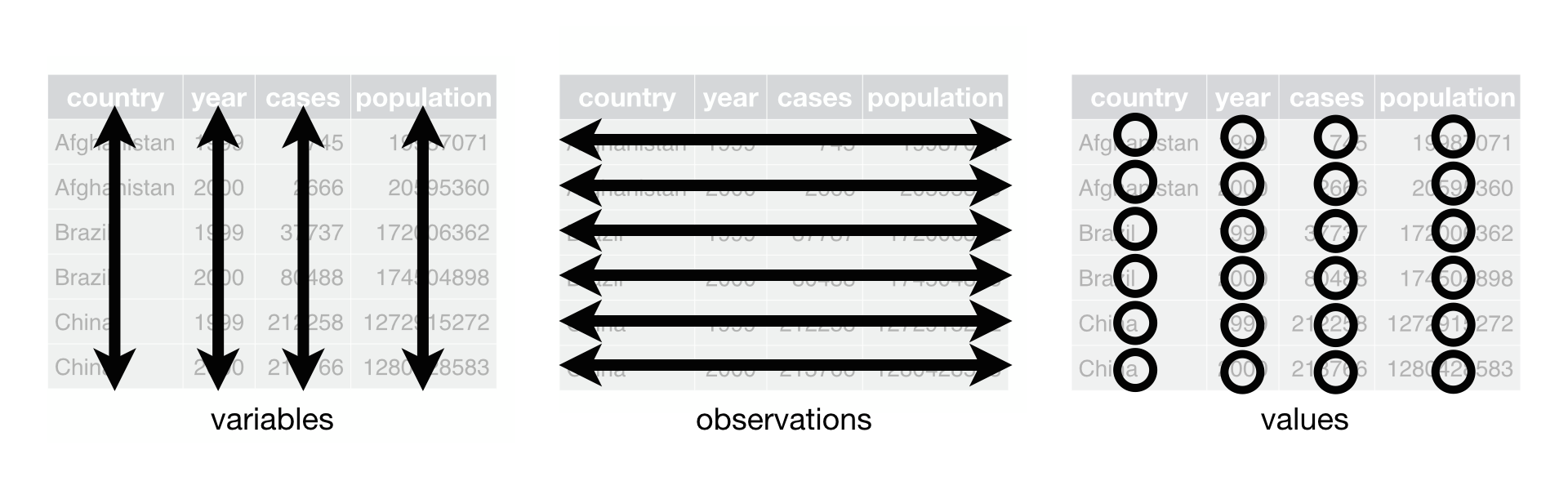
A good practice in R is to tidy your data. R follows a set of conventions that makes one layout of tabular data much easier to work with than others. Your data will be easier to work with in R if it follows three rules:
Each variable in the data set is placed in its own column
Each observation is placed in its own row
Each value is placed in its own cell
Illustration of tidy data.
Data that satisfies these rules is known as tidy data: you see that thanks to this representation, a 2D table can handle an arbitrary number of variables – this avoids using multi-dimensional arrays or multi-tab Excel documents. Note that it does’t matter if a value is repeated in a column.
Here is an example:
df<-read.csv("Data/population.csv")df# is not tidy
Understanding long and wide data with an animation. Source: tidyexplain
6.4.2 Tibbles
A tibble is an enhanced version of the data.frame provided by the tibble package (which is part of the tidyverse). The main advantage of tibble is that it has easier initialization and nicer printing than data.frame.
Moreover, the performance are also enhanced for the reading from files with read_csv(), read_tsv(), read_table() and read_delim() that do the same things as their read.xx() counterparts and return a tibble. Otherwise, the handling is basically the same.
Note that when initializing tibbles, the construction is iterative. It means that when creating a second column, one can refer to the first one that was created. This does’t work with data.frames.
# won't work unless a `x` vector was created beforedata.frame(x=runif(1e3), y=cumsum(x))
Tibbles are quite strict about subsetting. [ always returns another tibble. Contrast this with a data frame: sometimes [ returns a data frame and sometimes it just returns a vector:
Unless you want to get a tibble, I recommend always using the $ notation when you want to get a column as a vector to avoid problems.
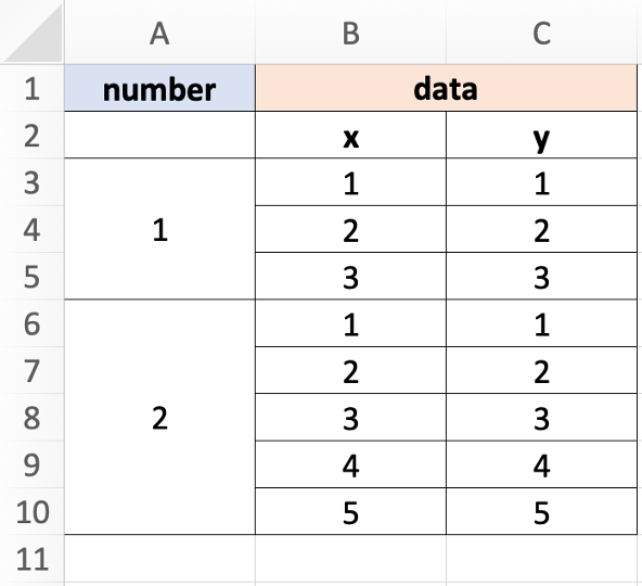
Another interesting feature of tibbles is that their columns can contain vectors, like usual, but also lists of any R objects like other tibbles, nls() objects, etc. This is called “nesting”, and you can nest and un-nest tibbles using these explicit functions:
tib_unnested_renested$data# The `data` column is a list
#> [[1]]
#> # A tibble: 2 × 2
#>   number     y
#>    <int> <int>
#> 1      1     1
#> 2      2     1
#>
#> [[2]]
#> # A tibble: 2 × 2
#>   number     y
#>    <int> <int>
#> 1      1     2
#> 2      2     2
#>
#> [[3]]
#> # A tibble: 2 × 2
#>   number     y
#>    <int> <int>
#> 1      1     3
#> 2      2     3
#>
#> [[4]]
#> # A tibble: 1 × 2
#>   number     y
#>    <int> <int>
#> 1      2     4
#>
#> [[5]]
#> # A tibble: 1 × 2
#>   number     y
#>    <int> <int>
#> 1      2     5
6.5 Operations in the tidyverse
In the end, base R and the tidyverse package provide many efficient functions to perform most of the tasks you would want to perform recursively, thus allowing avoiding explicit for loops (that are slow).
Here are some examples, and you will find much more here. Take a look at the cheatsheets on tidyr and on dplyr, it’s really helpful.
Let’s work on this tibble:
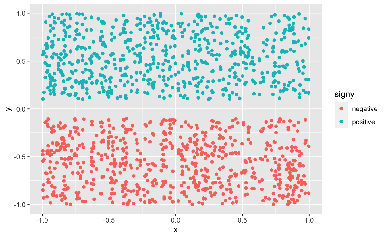
# Let's create a random tibblelibrary(tidyverse)N<-500dt<-tibble(x =rep(runif(N, -1, 1), 3), y =runif(N*3, -1, 1), signx =ifelse(x>0, "positive", "negative"), signy =ifelse(y>0, "positive", "negative"))dt
In the following, we will introduce the pipe operator |>, that was introduced in the version 4.1 of R. This operator allows a clear syntax for successive operations, as “what is on the left of the operator is given as first argument of what is on the right”. It is thus a good habit to write each operation on a separate line to facilitate the reading. This is particularly helpful when performing multiple nested operations. For example, summary(head(tail(dt),2)), which is hard to read, would translate to:
Note that before the 4.1 version of R, the pipe operator was only present thanks to the magrittr package, and was written %>%. In magrittr’s pipe, retrieving the piped object is done with the operator ., while it is done with the operator _ in base R’s.
Silly example:
"Hello"|>gsub("o", "e")# replace the substring "Hello" by "o" in string "e"
#> [1] "e"
"Hello"|>gsub("o", "e", x=_)# replace the substring "o" by "e" in string "Hello"
#> [1] "Helle"
"Hello"%>%gsub("o", "e")# replace the substring "Hello" by "o" in string "e"
#> [1] "e"
# /!\ In base R pipe, the '_' needs to be for a named argument, # while it is not necessary for the '%>%' pipe"Hello"%>%gsub("o", "e", .)# replace the substring "o" by "e" in string "Hello"
group_by(column) groups by similar values of the wanted column(s) and performs the next operations on each element of the group successively.
Alternatively, you can use the parameter by=column or .by=column in the functions you want to use on groups. The difference between group_by(column) and .by=column is that after group_by(column), the tibble stays grouped – so an ungroup() is needed to remove the grouping.
At least one column with the exact same name must be present in each table to use the xx_join() functions. There are more possibilities than inner_join() that I show here, see the help for more information.
The separation is based on standard separators such as “-”, “_”, “.”, ” “, etc. A single separator can be specified with the argument sep, otherwise all separators are used. One must provide the resulting vector of new column names: if one value is NA, this column will be discarded. Examples:
6.5.13 Apply a function recursively on each element of a column
Take a look at the cheatsheet on the purrr package for more options and a visual help on the map() family. I show here a use of purrr::map(vector, function) that returns a list. map(x, f) applies the function f() to each element of the vector x, putting the result in a separate element of a list: map(x, f) ->list(f(x1), f(x2), ... f(xn)). In case f(xi) returns a single value, you might want to use map_dbl() or map_chr(), for example, that will return a vector of doubles or of characters, respectively.
You see that you can create the function directly within the call to map using the shortcut map(vector, ~function(.)). This is useful to provide more arguments to the function – another solution is to write your own function before the call to map() and then call this function in map().
Note that in case you need more parameters, you can use purrr::map2(vector1, vector2, ~function(.x, .y)), where .x and .y refer to vector1 and vector2, respectively (it’s always .x and .y whatever the name of vector1 and vector2).
Create a 3 column data.frame containing 10 random values, their sinus, and the sum of the two first columns.
Print the 4 first lines of the table
Print the second column
Print the average of the third column
Using plot(x,y) where x and y are vectors, plot the 2nd column as a function of the first
Look into the function write.table() to write a text file containing this data.frame
Do the all the same things with a tibble
Solution
# Create a 3 column `data.frame`{.R} containing 10 random values, their sinus, # and the sum of the two first columns.x<-runif(10)y<-sin(x)z<-x+ydf<-data.frame(x=x, y=y, z=z)# Print the 4 first lines of the tablehead(df, 4)
#>            x          y         z
#> 1 0.62483524 0.58496365 1.2097989
#> 2 0.36899686 0.36068000 0.7296769
#> 3 0.69465978 0.64012409 1.3347839
#> 4 0.07386248 0.07379534 0.1476578
# Look into the function `write.table()`{.R} to write a text file # containing this `data.frame`{.R}write.table(df, "Data/some_data.dat", quote =FALSE, row.names =FALSE)# # # # # # # # # # # # # # # # # # Tibble versionlibrary(tidyverse)df_tib<-tibble(a =runif(10), b =sin(a), c =a+b)head(df_tib, 4)
#> # A tibble: 4 × 3
#>       a     b     c
#>   <dbl> <dbl> <dbl>
#> 1 0.199 0.198 0.397
#> 2 0.523 0.499 1.02
#> 3 0.814 0.727 1.54
#> 4 0.642 0.599 1.24
Create a subset containing the data for Montpellier
What is the max and min of population in this city?
The average population over time?
What is the total population in 2012?
What is the total population per year?
What is the average population per city over the years?
Solution
# Download population.txt and load it into a `data.frame`{.R}.library(tidyverse)popul<-read_csv("Data/population.csv")# What are the names of the columns and the dimension of the table?names(popul); dim(popul)
# Create a subset containing the data for Montpelliermtp<-subset(popul.tidy, city=="Montpellier")# I prefer the tidyverse versionmtp<-popul.tidy|>filter(city=="Montpellier")# What is the max and min of population in this city?max(mtp$pop)
Create a new tibble pp by using the pipe operator (%>%) and successively:
joining the two tibbles into one using inner_join()
adding a column age containing the age in years (use lubridate::time_length(x, 'years') with x a time difference in days) by using mutate()
Display a summary of the table using str()
Using groupe_by() and summarize():
Show the number of males and females in the table (use the counter n())
Show the average age per gender
Show the average size per gender and institution
Show the number of people from each country, sorted by descending population (arrange())
Using select(), display:
only the name and age columns
all but the name column
Using filter(), show data only for
Chinese people
From institution ECL and UCBL
People older than 22
People with a e in their name
Solution
# First, load the `tidyverse` packagelibrary(tidyverse)# Load people1.csv and people2.csvpp1<-read_csv("Data/people1.csv")pp2<-read_csv("Data/people2.csv")# Create a new tibble `pp` by using the pipe operator (`%>%`)# and successively:# - joining the two tibbles into one using `inner_join()`# - adding a column `age` containing the age in years # (use lubridate's `time_length(x, 'years')` with x a time# difference in days) by using `mutate()`pp<-pp1|>inner_join(pp2)|>mutate(age=time_length(today()-dateofbirth,'years'))# Display a summary of the table using `str()`str(pp)
# Using `groupe_by()` and `summarize()`:# - Show the number of males and females in the table # (use the counter `n()`)pp|>group_by(gender)|>summarize(count=n())
# Data frames## Defining a data.frame### Defining a data.frame from vectorsIn R, the principal object is *the data*. Hence the `data.frame`{.R} object, which is basically a table of vectors. A `data.frame`{.R} is a list presented under the form of a table – *i.e.* a spreadsheet. On a day-to-day basis, you will either define `data.frame`{.R} from existing vectors or other `data.frame`{.R}, or define a `data.frame`{.R} from a file (text, Excel...). In this example, we use <a href="Data/test.dat" download target="_blank">test.dat</a> and <a href="Data/test.xlsx" download target="_blank">test.xlsx</a>.To define a `data.frame` from known vectors, we just have to do:```{r, warnings=FALSE, message=FALSE}x <- seq(-pi, pi, length = 6) y <- sin(x)df <- data.frame(x, y) # df is a data.frame (a table)df```Then some information about our table are readily accessible, like:- The dimension, the number of rows and columns:```{r, warnings=FALSE, message=FALSE}dim(df); nrow(df); ncol(df)```- Print the first and last 3 values```{r, warnings=FALSE, message=FALSE}head(df, 3); tail(df, 3)```- Print some information on `df````{r, warnings=FALSE, message=FALSE}str(df)```- Print some statistics on `df````{r, warnings=FALSE, message=FALSE}summary(df)```If not defined when creating the `data.frame`, the column names will be by default the vector names. To specify your own column names, do it when creating the `data.frame`:```{r}df <-data.frame(xxx = x, yyy = y)head(df, 2)```Or, once it's created, do it using `names()`{.R}```{r}names(df)names(df) <-c("X", "Y")head(df, 2)```### Defining a data.frame from a file#### A text fileLet's say we have `test.dat` that looks like this:```{bash}# Bash code:head Data/test.dat```- Then, to read this file into a `data.frame`, we will use `read.table()`{.R}. If you don't specify that the file contains a header, `read.table()`{.R} will default to attributing column names that will be V1, V2, V3, etc:```{r}read.table("Data/test.dat")```- If your file contains column names, you can use the first line as column names, like so:```{r}read.table("Data/test.dat", header=TRUE)```- If you want to skip some lines before starting the reading, use `skip`:```{r}read.table("Data/test.dat", skip=1)```- You can specify your own column names using `col.names`:```{r}read.table("Data/test.dat", skip=1, col.names =c("A","B"))```- You can type `?read.table` for more options.#### An Excel fileNow, to read an Excel file, use the `readxl` library:```{r}library(readxl) # load readxl from tidyverse to read Excel filesread_excel("Data/test.xlsx", sheet=1)read_excel("Data/test.xlsx", sheet=2)```--- ## Accessing values - Like with vectors, accessing values is done using the `[]` notation, except that here there are two indexes: `df[row, column]`:```{r, warnings=FALSE}df[3,1]```- In general however, what you want is to access a given column, by its index:```{r, warnings=FALSE}df[,1]df[[1]]# this is a vector too```- Or, **preferably**, by its name using the `$` notation:```{r, warnings=FALSE}df$X```- Finally, you may want to apply filters on your table:```{r, warnings=FALSE}df[df$X < 0, ]```- Using the function `subset()`{.R}, the conditions are applied on column names (no need for `df$col_name` here, while you need it in the above expression):```{r, warnings=FALSE}subset(df, X>1)subset(df, X>1, select = c(X))```---## Adding columns or rows### Adding columns- To add a column, just attribute a value to an column that do not exist yet, it will be created:```{r, warnings=FALSE}# Adding columnsdf <- data.frame(x,y)df$z <- df$x^2df```- You can also create a `data.frame` of a `data.frame`:```{r, warnings=FALSE}data.frame(df, z=df$x^2, u=cos(df$x))```- Finally, you can use the `cbind()`{.R} function to bind two `data.frame` column-wise:```{r, warnings=FALSE}df2 <- data.frame(a = 1:length(x), b = 1:length(x))cbind(df, df2)```### Adding rowsFor this, use the `rbind()`{.R} function.:::{.callout-warning}## AttentionThe two `data.frame` must have the same number of columns _**and**_ the same column names.:::```{r, warnings=FALSE}rbind(df, df)```### Deleting rows/columnsThis works like with vectors:```{r, warnings=FALSE}df[-1,]df[,-1]```---## Tidy up!### What is tidy data?**A good practice in R is to *tidy* your data.** R follows a set of conventions that makes one layout of tabular data much easier to work with than others. Your data will be easier to work with in R if it follows three rules:- Each variable in the data set is placed in its own column- Each observation is placed in its own row- Each value is placed in its own cell```{r tidy, echo=FALSE, fig.cap="Illustration of tidy data.", fig.align="center", out.width="100%"}knitr::include_graphics("./Plots/tidy.png")```Data that satisfies these rules is known as tidy data: you see that thanks to this representation, a 2D table can handle an arbitrary number of variables – this avoids using multi-dimensional arrays or multi-tab Excel documents. Note that it does't matter if a value is repeated in a column. Here is an example:```rdf <-read.csv("Data/population.csv")df # is not tidy```<details> <summary>Show output</summary>```{r echo=FALSE}df <- read.csv("Data/population.csv")df # is not tidy```</details><br>```rlibrary(tidyr)df <-pivot_longer(df, cols=-year, names_to="city", values_to="pop")df #is tidy```<details> <summary>Show output</summary>```{r echo=FALSE, message=FALSE}library(tidyr)df <- pivot_longer(df, cols=-year, names_to="city", values_to="pop")df #is tidy```</details><br>```r# is not tidypivot_wider(df, names_from="city", values_from="pop")```<details> <summary>Show output</summary>```{r echo=FALSE}# is not tidypivot_wider(df, names_from="city", values_from="pop")```</details><br>You can find more information on data import and [tidyness](https://garrettgman.github.io/tidying/) on the [data-import cheatsheet](https://github.com/rstudio/cheatsheets/blob/main/data-import.pdf) and on the [tidyr](http://www.sthda.com/english/wiki/tidyr-crucial-step-reshaping-data-with-r-for-easier-analyses) package.```{r pivotgif, echo = FALSE, fig.cap = "Understanding long and wide data with an animation. Source: [tidyexplain](https://github.com/gadenbuie/tidyexplain)", fig.align="center", out.width="70%"}knitr::include_graphics('./Plots/tidyr-pivoting.gif')```### TibblesA `tibble`{.R} is an enhanced version of the `data.frame`{.R} provided by the `tibble` package (which is part of the `tidyverse`). The main advantage of `tibble`{.R} is that it has easier initialization and nicer printing than `data.frame`{.R}. Moreover, the performance are also enhanced for the reading from files with `read_csv()`{.R}, `read_tsv()`{.R}, `read_table()`{.R} and `read_delim()`{.R} that do the same things as their `read.xx()` counterparts and return a `tibble`. Otherwise, the handling is basically the same.More on tibbles [here](https://cran.r-project.org/web/packages/tibble/vignettes/tibble.html).```{r, include=FALSE}rm(x)```- Note that when initializing `tibble`s, the construction is iterative. It means that when creating a second column, one can refer to the first one that was created. This does't work with `data.frame`s.```{r, error=TRUE, warnings=FALSE, message=FALSE}# won't work unless a `x` vector was created beforedata.frame(x=runif(1e3), y=cumsum(x)) library(tidyverse)tib <- tibble(x=runif(1e3), y=cumsum(x))tib```:::{.callout-warning}## Attention:::`Tibble`s are quite strict about subsetting. `[` always returns another `tibble`. Contrast this with a data frame: sometimes `[` returns a data frame and sometimes it just returns a vector:```{r}head(tib[[1]]) # is a vectorhead(tib[,1]) # is a tibble```Unless you want to get a `tibble`, I recommend always using the `$` notation when you want to get a column as a vector to avoid problems.- Another interesting feature of `tibble`s is that their columns can contain vectors, like usual, but also lists of any R objects like other tibbles, `nls()`{.R} objects, etc. This is called "nesting", and you can nest and un-nest `tibble`s using these explicit functions:```{r warning=FALSE, message=FALSE}tib1 <- tibble(x=1:3, y=1:3)tib2 <- tibble(x=1:5, y=1:5)tib <- tibble(number=1:2, data=list(tib1, tib2))tib``````{r}#| label: fig-excel-nested#| echo: false#| fig-cap: "Excel equivalent to a nested `tibble`."#| out-width: 50%knitr::include_graphics("./Plots/excel-nested.png")``````{r warning=FALSE, message=FALSE}tib_unnested <- unnest(tib, data)tib_unnestedtib_unnested_renested <- nest(tib_unnested, data = c(number, y))tib_unnested_renestedtib_unnested_renested$data # The `data` column is a list```---## Operations in the tidyverseIn the end, base R and the `tidyverse` package provide many efficient functions to perform most of the tasks you would want to perform recursively, thus allowing avoiding explicit for loops (that are slow).Here are some examples, and you will find much more [here](https://cran.r-project.org/web/packages/dplyr/vignettes/dplyr.html). Take a look at the cheatsheets on [tidyr](https://github.com/rstudio/cheatsheets/blob/main/data-import.pdf) and on [dplyr](https://github.com/rstudio/cheatsheets/blob/main/data-transformation.pdf), it's really helpful. Let's work on this `tibble`:```{r, message=FALSE}# Let's create a random tibblelibrary(tidyverse)N <- 500dt <- tibble(x = rep(runif(N, -1, 1), 3), y = runif(N*3, -1, 1), signx = ifelse(x>0, "positive", "negative"), signy = ifelse(y>0, "positive", "negative"))dt```### The pipe operatorIn the following, we will introduce the pipe operator `|>`{.R}, that was introduced in the version 4.1 of R.This operator allows a clear syntax for successive operations, as "what is on the left of the operator is given as first argument of what is on the right". It is thus a good habit to write each operation on a separate line to facilitate the reading. This is particularly helpful when performing multiple nested operations. For example, `summary(head(tail(dt),2))`{.R}, which is hard to read, would translate to:```rdt |>tail() |>head(2) |>summary()```Note that before the 4.1 version of R, the pipe operator was only present thanks to the `magrittr` package, and was written `%>%`{.R}. In `magrittr`'s pipe, retrieving the piped object is done with the operator `.`, while it is done with the operator `_` in base R's.Silly example:```{r, error=TRUE}"Hello" |> gsub("o", "e") # replace the substring "Hello" by "o" in string "e""Hello" |> gsub("o", "e", x=_) # replace the substring "o" by "e" in string "Hello""Hello" %>% gsub("o", "e") # replace the substring "Hello" by "o" in string "e"# /!\ In base R pipe, the '_' needs to be for a named argument, # while it is not necessary for the '%>%' pipe"Hello" %>% gsub("o", "e", .) # replace the substring "o" by "e" in string "Hello"```### Sampling data```{r, message=FALSE}dt |> slice(1:3) # by indexdt |> slice_sample(n=3) # randomly```### Operations on groups of a variable`group_by(column)`{.R} groups by similar values of the wanted column(s) and performs the next operations on each element of the group successively.Alternatively, you can use the parameter `by=column`{.R} or `.by=column`{.R} in the functions you want to use on groups. The difference between `group_by(column)`{.R} and `.by=column`{.R} is that after `group_by(column)`{.R}, the tibble stays grouped – so an `ungroup()`{.R} is needed to remove the grouping.```{r, message=FALSE}dt |> group_by(signx)dt |> group_by(signx) |> slice_sample(n=3)dt |> group_by(signx, signy) |> slice_sample(n=3)dt |> slice_sample(by = c(signx, signy), n = 3)dt |> group_by(signx, signy) |> slice_sample(n=3) |> ungroup()```### Summary by groups of a variable`summarise()`{.R} returns a **single value** for each element of the groups.```{r, message=FALSE}dt |> group_by(signx) |> summarise(count = n(), mean_x = mean(x), sd_x = sd(x))dt |> group_by(signx, signy) |> summarise(count = n(), mean_x = mean(x), mean_y = mean(y))```### Sorting```{r, message=FALSE}dt |> arrange(x)dt |> arrange(x, desc(y))```### Merge tables column-wiseAt least one column with the **exact** same name must be present in each table to use the `xx_join()`{.R} functions. There are more possibilities than `inner_join()`{.R} that I show here, see the help for more information.```{r, message=FALSE}dt2 <- tibble(signx=c("positive","positive","negative","negative"), signy=c("positive","negative","positive","negative"), value=c(TRUE, FALSE, FALSE, TRUE))dt2inner_join(dt, dt2)```### Merge tables row-wiseThis works even if there are missing rows.```{r, message=FALSE}dt3 <- tibble(a=1:3, b=3:5, c=6:8)dt4 <- tibble(a=3:1, c=3:5)bind_rows(dt3, dt4)```### Add/modify a column`mutate()`{.R}, like `$`{.R}, adds a column if it doesn't exist, and modifies it if it does.```{r, message=FALSE}dt |> mutate(w=seq_along(x), z=sin(x))dt |> mutate(x=seq_along(x))```### Selecting columns```{r, message=FALSE}dt |> select(x) # only xdt |> select(-x) # all but xdt |> select(starts_with("sign"))dt |> select(contains("x"))```### Filtering columns```{r, message=FALSE}dt |> filter(signx=="positive")dt |> filter(x<0, y>.1) # multiple filters can be applied at once```### Reorder columns```{r, message=FALSE}dt |> relocate(y, .after = signy)```### Separate columnsThe separation is based on standard separators such as "-", "\_", ".", " ", etc. A single separator can be specified with the argument `sep`, otherwise all separators are used. One must provide the resulting vector of new column names: if one value is `NA`{.R}, this column will be discarded. Examples:```{r, message=FALSE}dt5 <- tibble(file=list.files(path="Exo/FTIR/Data/", pattern=".xls"))dt5dt5 |> separate(file, c(NA, "sample", "temperature", NA), convert = TRUE)dt5 |> separate(file, c("name", "extension"), sep = "\\.")```### Apply a function recursively on each element of a columnTake a look at the [cheatsheet on the `purrr` package](https://github.com/rstudio/cheatsheets/blob/main/purrr.pdf) for more options and a visual help on the `map()` family. I show here a use of `purrr::map(vector, function)`{.R} that returns a list. `map(x, f)`{.R} applies the function `f()` to each element of the vector `x`, putting the result in a separate element of a list: `map(x, f) -> list(f(x1), f(x2), ... f(xn))`{.R}. In case `f(xi)` returns a single value, you might want to use `map_dbl()` or `map_chr()`, for example, that will return a vector of doubles or of characters, respectively.```{r, message=FALSE}x <- c(pi, pi/3, pi/2)map(x, sin) # returns a listx |> map_dbl(sin) # returns a vector```Of course, in the above case, it's a stupid use of the power of `map()`{.R}. A typical use case is when you want to read multiple files, for example:```{r, message=FALSE, warning=FALSE}dt6 <- tibble(file=list.files(path="Exo/spectro2/Data", pattern = ".txt", full.names = TRUE)) |> slice(1:5) |> mutate(data = map(file, read_table, col_names = c("w", "Int"))) |> mutate(file = basename(file))dt6```This is (almost) equivalent to:```{r, message=FALSE, warning=FALSE}dt6 <- tibble(file=list.files(path="Exo/spectro2/Data", pattern = ".txt", full.names = TRUE)) |> slice(1:5) |> mutate(data = map(file, ~read_table(., col_names = c("w", "Int")))) |> mutate(file = basename(file))```You see that you can create the function directly within the call to map using the shortcut `map(vector, ~ function(.))`{.R}. This is useful to provide more arguments to the function -- another solution is to write your own function before the call to `map()`{.R} and then call this function in `map()`{.R}.Note that in case you need more parameters, you can use `purrr::map2(vector1, vector2, ~function(.x, .y))`{.R}, where `.x` and `.y` refer to `vector1` and `vector2`, respectively (it's always `.x` and `.y` whatever the name of `vector1` and `vector2`).```{r}tibble(x=1:3, y=5:7) |>mutate(sum =map2_dbl(x, y, sum))tibble(a=list(tibble(x=1:3, y=5:7), tibble(x=0:3, y=4:7)), b=list(tibble(x=10:13, y=15:18), tibble(x=-1:2, y=-14:-17))) |>mutate(sumx =map2_dbl(a, b, ~sum(.x$x, .y$x)),sumy =map2_dbl(a, b, ~sum(.x$y, .y$y)))```### Nesting and un-nesting data```{r, message=FALSE}dt7 <- dt6 |> mutate(file = basename(file)) |> unnest(data)dt7# Nesting data per repeated values in a column (~equivalent to grouping)dt7 |> nest(data=-file)```### Providing data to ggplot```{r, message=FALSE}dt |> filter(abs(y) > 0.1) |> ggplot(aes(x=x, y=y, color=signy))+ geom_point()```## Exercises {#exo-df}Download the exercises and solutions from the following repositories, then create a Rstudio project from the unzipped folder:- [Beginner exercises](https://github.com/colinbousige/R1-beginner)- [Advanced exercises](https://github.com/colinbousige/R2-advanced)---<details> <summary>**Exercise 1**</summary>- Create a 3 column `data.frame`{.R} containing 10 random values, their sinus, and the sum of the two first columns.- Print the 4 first lines of the table- Print the second column- Print the average of the third column- Using `plot(x,y)`{.R} where `x` and `y` are vectors, plot the 2nd column as a function of the first- Look into the function `write.table()`{.R} to write a text file containing this `data.frame`{.R}- Do the all the same things with a `tibble`{.R}<details> <summary>Solution</summary>```{r, warnings=FALSE}# Create a 3 column `data.frame`{.R} containing 10 random values, their sinus, # and the sum of the two first columns.x <- runif(10)y <- sin(x)z <- x + ydf <- data.frame(x=x, y=y, z=z)# Print the 4 first lines of the tablehead(df, 4)# Print the second columndf[,2]# Print the average of the third columnmean(df$z); mean(df[3]); mean(df[,3])# Using `plot(x,y)`{.R} where `x` and `y` are vectors, # plot the 2nd column as a function of the firstplot(df[,1], df[,2])plot(df$x, df$y)# Look into the function `write.table()`{.R} to write a text file # containing this `data.frame`{.R}write.table(df, "Data/some_data.dat", quote = FALSE, row.names = FALSE)# # # # # # # # # # # # # # # # # # Tibble versionlibrary(tidyverse)df_tib <- tibble(a = runif(10), b = sin(a), c = a + b)head(df_tib, 4)df_tib[,2]; df_tib[[2]];mean(df_tib$c); mean(df_tib[3]); mean(df_tib[,3]); mean(df_tib[[3]])write.table(df_tib, "Data/some_data.dat", quote = FALSE, row.names = FALSE)plot(df_tib$a, df_tib$b)```</details></details><details> <summary>**Exercise 2**</summary>- Download the files: - <a href="Data/rubis_01.txt" download target="_blank">rubis_01.txt</a> - <a href="Data/population.csv" download target="_blank">population.csv</a> - <a href="Data/FTIR_rocks.xlsx" download target="_blank">FTIR_rocks.xlsx</a>- Load them into separate `data.frames`{.R}. Look into the options of `read.table()`{.R}, `read.csv()`{.R}, `readxl::read_excel()`{.R}, to get the proper data fields.- Add column names to the data.frame containing `rubis_01.txt`. - Print their dimensions.- Do the same things with tibbles.<details> <summary>Solution</summary>```{r, warnings=FALSE, message=FALSE}rubis_01 <- read.table("Data/rubis_01.txt", col.names = c("w", "intensity"))population <- read.csv("Data/population.csv")FTIR_rocks <- readxl::read_excel("Data/FTIR_rocks.xlsx")dim(rubis_01); names(rubis_01)dim(population); names(population)dim(FTIR_rocks); names(FTIR_rocks)library(tidyverse)rubis_01 <- read_table("Data/rubis_01.txt", col_names = c("w", "intensity"))population <- read_csv("Data/population.csv")```</details></details><details> <summary>**Exercise 3**</summary>- Download the TGA data file <a href="Data/ATG.txt" download target="_blank">ATG.txt</a>- Load it into a `data.frame`{.R}. Look into the options of `read.table()`{.R} to get the proper data fields.- Do the same with a tibble<details> <summary>Solution</summary>```{r}d <-read.table("Data/ATG.txt", skip=12,header=FALSE, nrows=4088)names(d) <-c("Index", "t", "Ts", "Tr", "Value")head(d)d <-read.table("Data/ATG.txt", skip=10,comment.char="[",header=TRUE, nrows=4088)head(d)library(tidyverse)d <-read_table("Data/ATG.txt", skip =10,comment ="[") |>drop_na()d```</details></details><details> <summary>**Exercise 4**</summary>Download <a href="Data/population.csv" download target="_blank">population.csv</a> and load it into a `tibble`{.R}.- What are the names of the columns?- Are the data tidy? make the table tidy if needed- Create a subset containing the data for Montpellier + What is the max and min of population in this city? + The average population over time?- What is the total population in 2012?- What is the total population per year?- What is the average population per city over the years?<details><summary>Solution</summary>```{r}# Download population.txt and load it into a `data.frame`{.R}.library(tidyverse)popul <-read_csv("Data/population.csv")# What are the names of the columns and the dimension of the table?names(popul); dim(popul)# Are the data tidy?head(popul) # nopopul.tidy <- popul |>pivot_longer(cols=-year,names_to ="city",values_to ="pop" )popul.tidy# Create a subset containing the data for Montpelliermtp <-subset(popul.tidy, city =="Montpellier")# I prefer the tidyverse versionmtp <- popul.tidy |>filter(city =="Montpellier")# What is the max and min of population in this city?max(mtp$pop)min(mtp$pop)range(mtp$pop)# The average population over time?mean(mtp$pop)# What is the total population in 2012?sum(popul.tidy[popul.tidy$year ==2012, "pop"])popul.tidy |>filter(year==2012) |>select(pop) |>sum()# What is the total population per year?popul.tidy |>group_by(year) |>summarise(pop_tot=sum(pop))# What is the average population per city over the years?popul.tidy |>group_by(city) |>summarise(pop_ave=mean(pop))```</details></details><details> <summary>**Exercise 5**</summary>- First, load the `tidyverse` and `lubridate` package- Load <a href="Data/people1.csv" download target="_blank">people1.csv</a> and <a href="Data/people2.csv" download target="_blank">people2.csv</a> into `pp1` and `pp2`- Create a new tibble `pp` by using the pipe operator (`%>%`{.R}) and successively: - joining the two tibbles into one using `inner_join()`{.R} - adding a column `age` containing the age in years (use `lubridate::time_length(x, 'years')`{.R} with x a time difference in days) by using `mutate()`{.R}- Display a summary of the table using `str()`{.R}- Using `groupe_by()`{.R} and `summarize()`{.R}: - Show the number of males and females in the table (use the counter `n()`{.R}) - Show the average age per gender - Show the average size per gender and institution - Show the number of people from each country, sorted by descending population (`arrange()`{.R})- Using `select()`{.R}, display: - only the name and age columns - all but the name column- Using `filter()`{.R}, show data only for - Chinese people - From institution ECL and UCBL - People older than 22 - People with a `e` in their name<details> <summary>Solution</summary>```{r, warnings=FALSE, message=FALSE}# First, load the `tidyverse` packagelibrary(tidyverse)# Load people1.csv and people2.csvpp1 <- read_csv("Data/people1.csv")pp2 <- read_csv("Data/people2.csv")# Create a new tibble `pp` by using the pipe operator (`%>%`)# and successively:# - joining the two tibbles into one using `inner_join()`# - adding a column `age` containing the age in years # (use lubridate's `time_length(x, 'years')` with x a time# difference in days) by using `mutate()`pp <- pp1 |> inner_join(pp2) |> mutate(age=time_length(today()-dateofbirth,'years'))# Display a summary of the table using `str()`str(pp)# Using `groupe_by()` and `summarize()`:# - Show the number of males and females in the table # (use the counter `n()`)pp |> group_by(gender) |> summarize(count=n())# - Show the average age per genderpp |> group_by(gender) |> summarize(age=mean(age))# - Show the average size per gender and institutionpp |> group_by(gender, institution) |> summarize(size=mean(size))# - Show the number of people from each country, # sorted by descending populationpp |> group_by(origin) |> summarize(count=n()) |> arrange(desc(count))# Using `select()`, display:# - only the name and age columnspp |> select(c(name, age))# - all but the name columnpp |> select(-name)# Using `filter()`, show data only for# - Chinese peoplepp |> filter(origin=='China')# - From institution ECL and UCBLpp |> filter(institution %in% c('ECL', 'UCBL'))# - People older than 22 pp |> filter(age>22)# - People with a `e` in their namepp |> filter(grepl('e',name))```</details>----For more interesting exercises in the tidyverse, look at:- [CO2 emissions: data wrangling and ggplot2](Exo/co2/exercise.html)- [Religion and babies: data handling, ggplot2 and plotly](Exo/religion_babies/exercise.html)- [COVID-19: data wrangling, ggplot2](Exo/covid/exercise.html)- [Nanoparticles statistics from SEM images: data wrangling, ggplot2 and fitting](Exo/SEM_particles/exercise.html)<br><br><br><br><br><br><br><br><br><br>