13 Fitting
13.1 What does it mean to “fit data”?
It might sound like a trivial question, but let’s make sure we’re all on the same page…
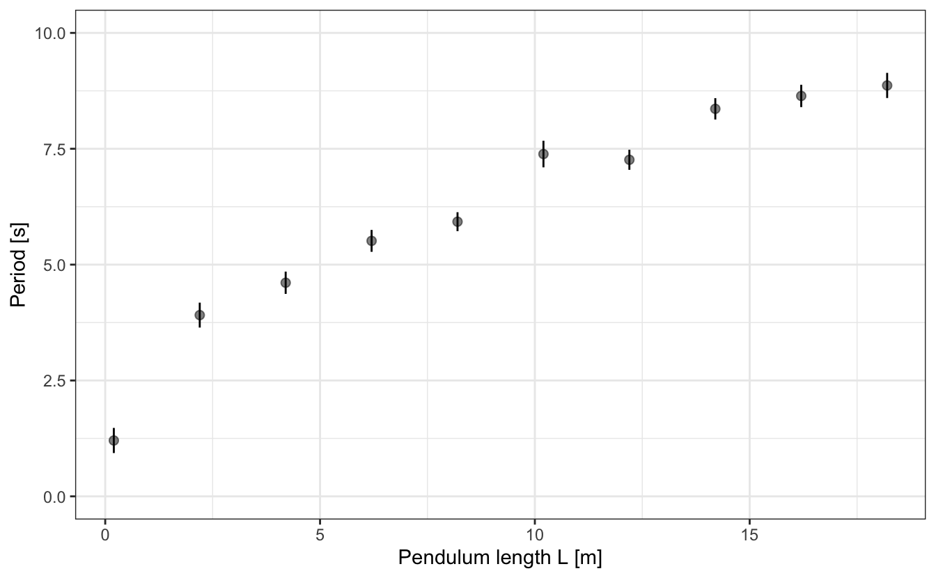
For the sake of the example, let’s take a look at some experimental measurements of the oscillation period T of a pendulum1. We have measured this period for various lengths L of the pendulum, and it results in such an evolution:
Now, if you recall your high school physics class, you might remember that the period of the pendulum T is given by:
\[ T \simeq 2\pi\sqrt{\frac{L}{g}}, \tag{13.1}\]
where L is the pendulum length and g the acceleration of gravity. Such and experimental design, i.e. measuring T as a function of L, is therefore a means to determining the value of g.
For this, we need to perform a fit of our experimental data by a physical model, i.e. the one of Equation 13.1. When doing so, one has to distinguish between:
- Variables: the period T and the pendulum length L are variables, they are the quantities that vary for a given parameter.
- Parameters: the gravity g is a parameter of the fit that we wish to determine, i.e. it is a constant for this set of measurements.
So now, what exactly is a fit? Fitting a model to experimental data means:
- Finding the model that best describe our data (a line, a Gaussian, a polynomial, Equation 13.1, etc.). You can try several models and compare them to determine which model is the best.
- Finding the set of parameters of the model that best describe our data. This is done through an optimization algorithm.
How do we know the parameters are the best ones to describe our data? For this, we use a tool called the residual error function, \(\chi^2\), such as:
\[ \chi^2=\sum_{i=1}^N\left(y_i(x_i)-m_i(x_i, \{p\})\right)^2, \] where \(y_i(x_i)\) are the N experimental observations of the value \(y\) as a function of \(x\), and \(m_i(x_i, \{p\})\) is the value of the model as a function of \(x\) and the ensemble of parameters \(\{p\}\). We use the squared sum of residuals and not the simple sum of residuals because the residuals can either be positive or negative, and we are interested in minimizing the total distance from our model to our experimental data.
Applied to our pendulum problem, we thus get:
\[ \chi^2=\sum_{i=1}^N\left(T_i-2\pi\sqrt{\frac{L_i}{g}}\right)^2, \] where the summation is performed on the N points that we have recorded in Figure 13.1. In this case there is only one parameter, but you will encounter other models needing more than one parameter (for example if you’re fitting a peak, you’ll need it’s position, width, and height: 3 parameters). The rule of thumb is that the less parameters you introduce the better, “less” being compared to the number of data points.
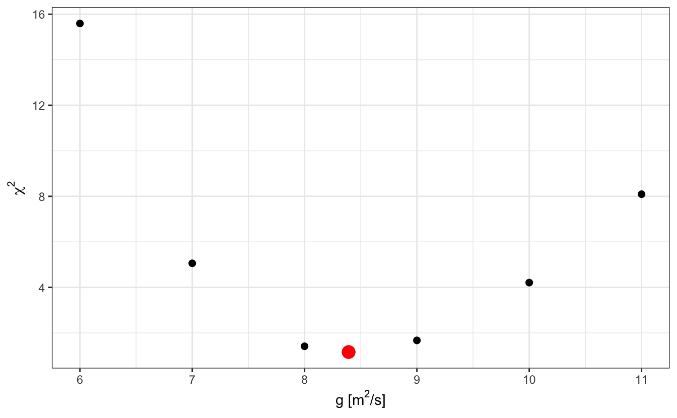
So, let’s try a few values of g and see what is the resulting residual error \(\chi^2\) in each case:
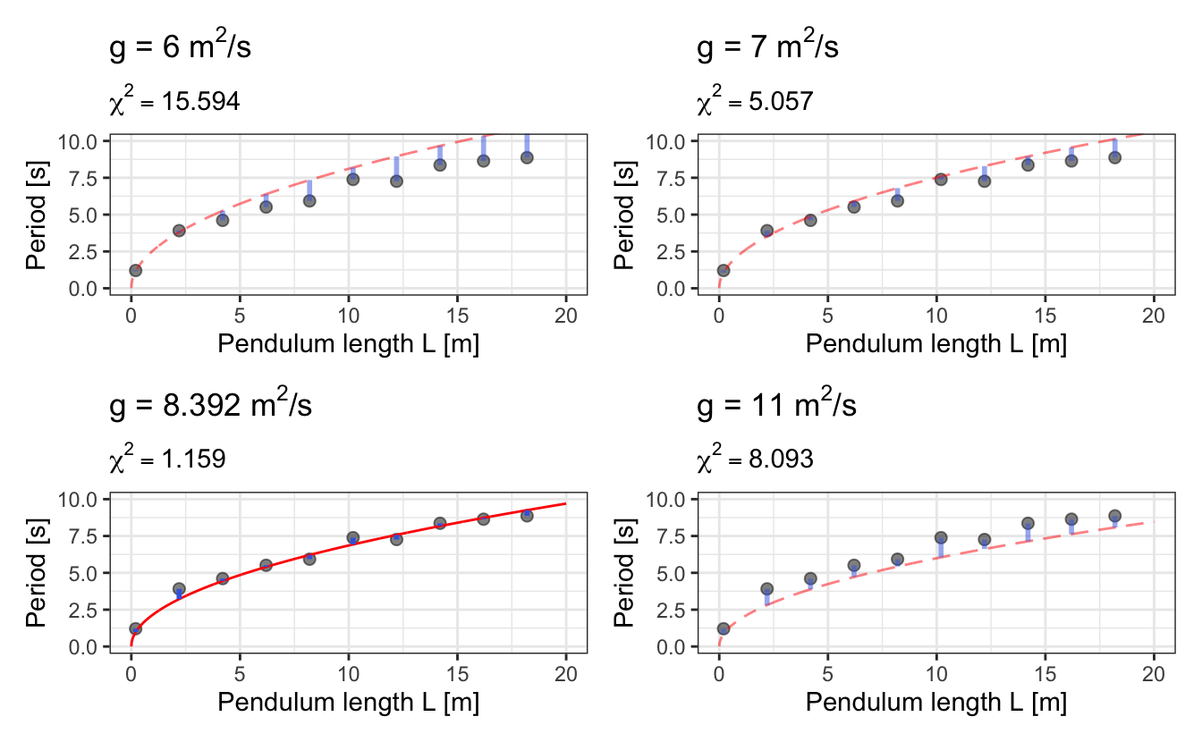
We see that there is a sweet spot in the values of g for which \(\chi^2\) is minimum:
Important
Fitting a model to experimental data is finding this sweet spot for the ensemble of parameters through an optimization procedure.
There are numerous algorithms out there to perform this optimization, but we will not delve into their mechanics.
Now, let’s get back to R. You will mainly use two functions to perform these optimizations:
Important
Note that, whenever it is possible, it is usually preferable to make your problem a linear one, as it avoids the hassle of providing starting values. For example, in the pendulum case above, taking the square of Equation 13.1 results in a linear evolution of \(T^2\) with respect to \(l\).
13.2 Linear fitting with lm()
Let’s learn how to do simple linear fits with R’s lm() and plot the results. Let’s start with some fake data stored in a tibble called d:
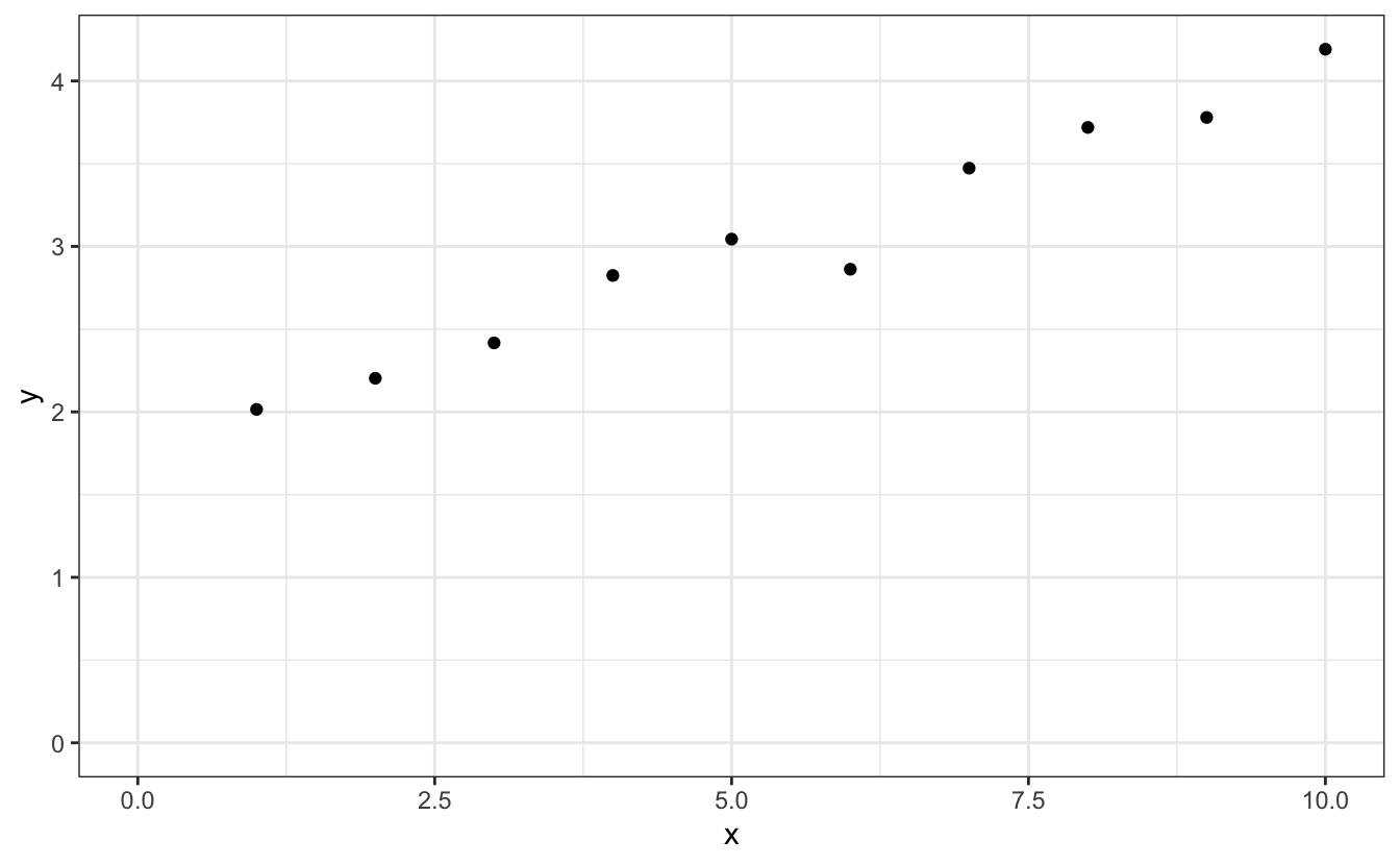
We see that this data shows a linear evolution, for which we might want to extract the slope and the intercept. This is very simply done by applying the lm() function, like so:
Here, and everywhere else in R, the operator ~ is to be understood as “as a function of”. So with this bit of code, we tell R to “fit y as a function of x using a linear model”.
Now to see the fit results, we can just display fit, or call summary(fit)
# Summary of the fit
fit
#>
#> Call:
#> lm(formula = y ~ x, data = d)
#>
#> Coefficients:
#> (Intercept) x
#> 1.75 0.23summary(fit)#>
#> Call:
#> lm(formula = y ~ x, data = d)
#>
#> Residuals:
#> Min 1Q Median 3Q Max
#> -0.21219 -0.02852 0.03580 0.06282 0.10676
#>
#> Coefficients:
#> Estimate Std. Error t value Pr(>|t|)
#> (Intercept) 1.75033 0.07486 23.38 1.19e-08 ***
#> x 0.23000 0.01206 19.07 5.93e-08 ***
#> ---
#> Signif. codes: 0 '***' 0.001 '**' 0.01 '*' 0.05 '.' 0.1 ' ' 1
#>
#> Residual standard error: 0.1096 on 8 degrees of freedom
#> Multiple R-squared: 0.9785, Adjusted R-squared: 0.9758
#> F-statistic: 363.5 on 1 and 8 DF, p-value: 5.933e-08To actually retrieve and store the fit parameters, call coef(fit):
# Retrieve the coefficients and errors
coef(fit)
#> (Intercept) x
#> 1.7503330 0.2300045coef(fit)[1]#> (Intercept)
#> 1.750333To get it properly stored in a tibble, see the broom package that we describe later in this chapter:
# Summary of the fit
broom::tidy(fit)
#> # A tibble: 2 × 5
#> term estimate std.error statistic p.value
#> <chr> <dbl> <dbl> <dbl> <dbl>
#> 1 (Intercept) 1.75 0.0749 23.4 0.0000000119
#> 2 x 0.230 0.0121 19.1 0.0000000593To get the standard error of the fitted parameters and the R2:
summary(fit)$coefficients#> Estimate Std. Error t value Pr(>|t|)
#> (Intercept) 1.7503330 0.07485606 23.38265 1.189474e-08
#> x 0.2300045 0.01206415 19.06513 5.932759e-08summary(fit)$coefficients["x", "Std. Error"]#> [1] 0.01206415summary(fit)$r.squared#> [1] 0.9784645And finally, to plot the result of the fit:
# Get the fitted paramters and make a string with it to be printed
to_print <- glue("y = {round(coef(fit)[1],2)} + x*{round(coef(fit)[2],2)}")
# Base plot
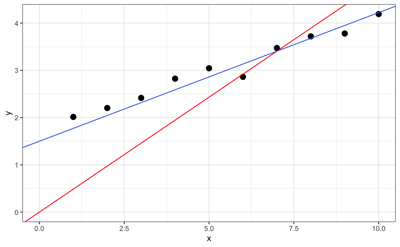
plot(d, pch = 16, main = "With base plot", sub = to_print)
abline(coef(fit), col="red")
# GGplot versions
ggplot(data=d, aes(x,y)) +
    geom_point(cex=3) +
    geom_abline(slope = coef(fit)[2], intercept = coef(fit)[1], col="red") +
    labs(title = "With ggplot and the parameters you get from the external call to lm()",
         subtitle = to_print)
ggplot(data=d, aes(x,y)) +
    geom_point(cex=3) +
    geom_smooth(method="lm") + # does the fit but does not allow saving the parameters
    labs(title = "With ggplot and the geom_smooth() function",
         subtitle = to_print)
The function geom_smooth() will fit the data and display the fitted line, but to retrieve the actual coefficients you still need to run lm().
Finally, you may want to impose an intercept that will be 0 or a given value. For this, you will need to add +0 in the formula, like so:
13.3 Nonlinear Least Squares fitting
13.3.1 The nls() workhorse
You can fit data with your own functions and constraints using nls(). Here is an example of data we may want to fit, stored into a tibble called df:
ggplot(data=df, aes(x,y))+
    geom_point()+
    ggtitle("Some fake data we want to fit with 2 Gaussians")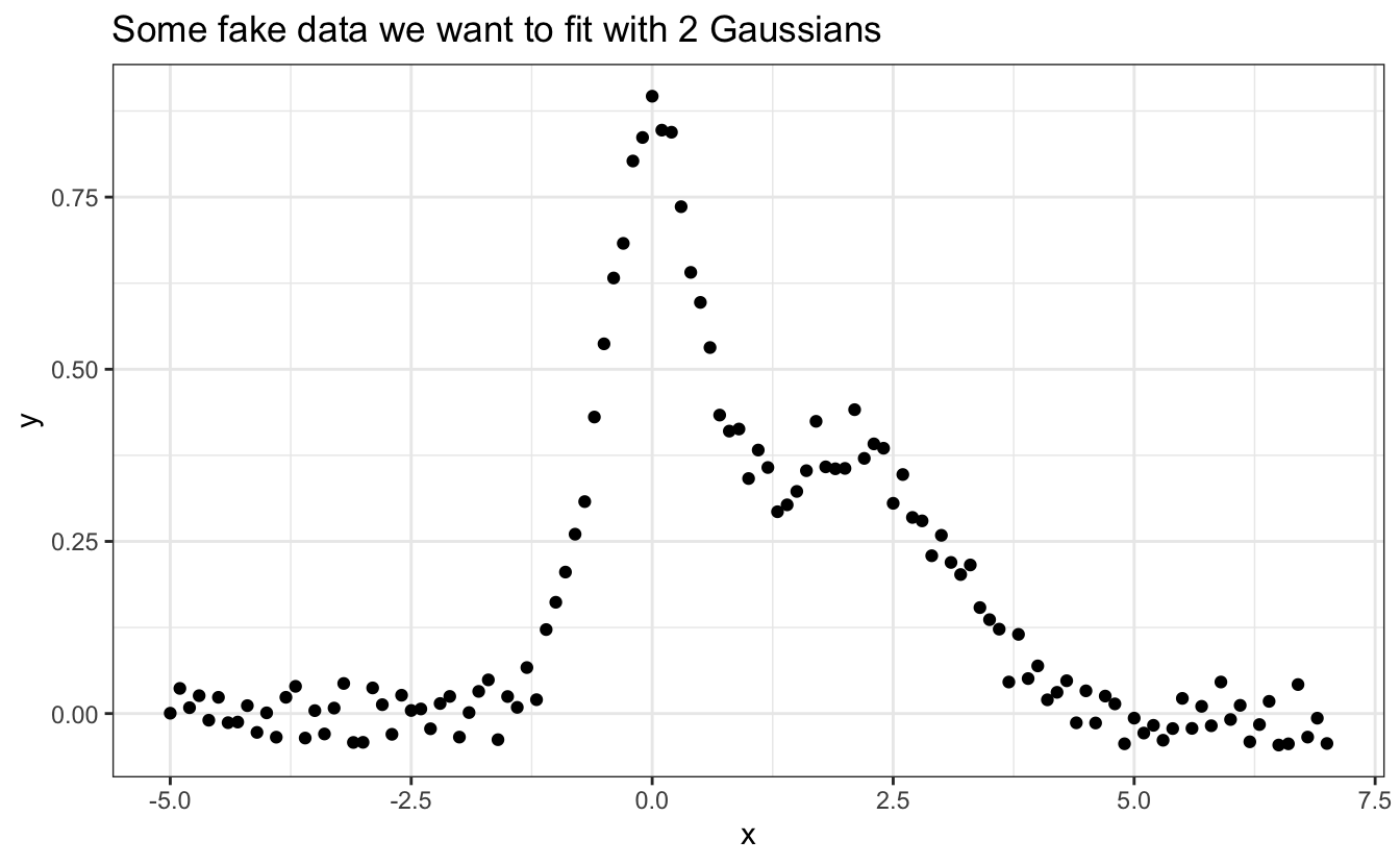
We first need to define a function to fit our data. We see here that it contains two peaks that look Gaussian, so let’s go with the sum of two Gaussian functions:
# Create a function to fit the data
myfunc <- function(x, y0, x1, x2, A1, A2, sd1, sd2) {
y0 + # baseline
A1 * dnorm(x, mean = x1, sd = sd1) +# 1st Gaussian
A2 * dnorm(x, mean = x2, sd = sd2) # 2nd Gaussian
}
# Fit the data using a user function
fit_nls <- nls(data=df,
y ~ myfunc(x, y0, x1, x2, A1, A2, sd1, sd2),
# Provide starting point for parameters values:
start = list(y0=0, x1=0, x2=1.5,
sd1=.2, sd2=.2,
A1=1, A2=1)
)
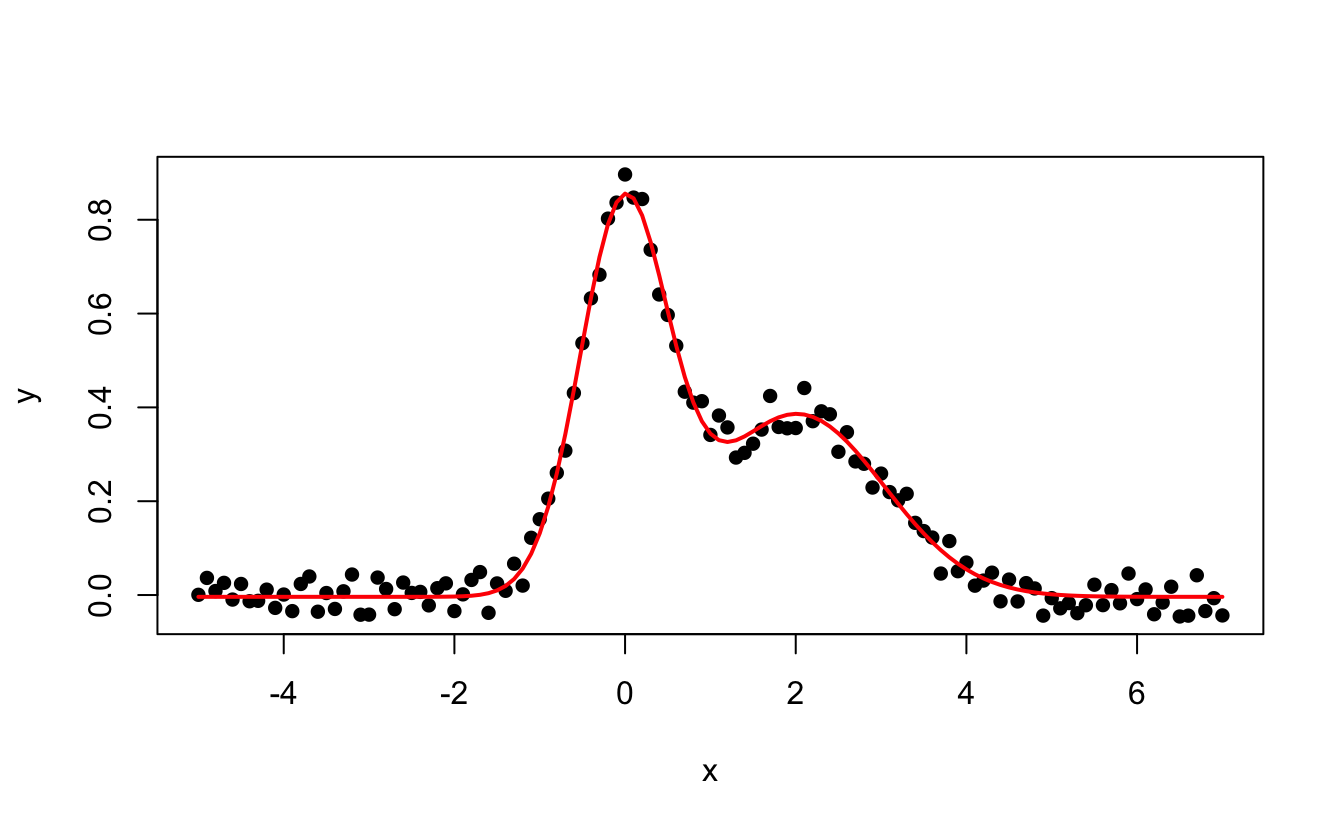
summary(fit_nls)#>
#> Formula: y ~ myfunc(x, y0, x1, x2, A1, A2, sd1, sd2)
#>
#> Parameters:
#> Estimate Std. Error t value Pr(>|t|)
#> y0 0.003066 0.003702 0.828 0.409
#> x1 0.001729 0.012639 0.137 0.891
#> x2 1.959162 0.046244 42.366 <2e-16 ***
#> sd1 0.497152 0.012364 40.209 <2e-16 ***
#> sd2 1.009802 0.047403 21.303 <2e-16 ***
#> A1 0.987399 0.035369 27.917 <2e-16 ***
#> A2 1.007223 0.045414 22.179 <2e-16 ***
#> ---
#> Signif. codes: 0 '***' 0.001 '**' 0.01 '*' 0.05 '.' 0.1 ' ' 1
#>
#> Residual standard error: 0.02923 on 114 degrees of freedom
#>
#> Number of iterations to convergence: 8
#> Achieved convergence tolerance: 6.411e-06And to plot the data and the result of the fit, we use predict(fit) to retrieve the fitted y values:
13.3.2 Using constraints
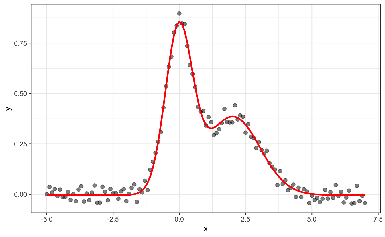
In nls() it is even possible to constraint the fitting by adding lower and upper boundaries. These boundaries are useful when you want to give some physical meaning to your parameters, for example, like forcing the width and amplitude to be positive or above a certain minimum value. However, you have to be careful with these and not provide stupid ones, e.g.:
# Constraining the upper and lower values of the fitting parameters
fit_constr <- nls(data = df,
                  y ~ myfunc(x, y0, x1, x2, A1, A2, sd1, sd2),
                  start = list(y0=0, x1=0, x2=3,
                               sd1=.2, sd2=.2, A1=1, A2=1),
                  upper = list(y0=Inf, x1=Inf, x2=Inf,
                               sd1=Inf, sd2=Inf, A1=2, A2=2),
                  lower = list(y0=-Inf, x1=-Inf, x2=2.9,
                               sd1=0, sd2=0, A1=0, A2=0),
                  algorithm = "port"
                 )
# Plotting the resulting function in blue
ggplot(data=df, aes(x,y))+
    ggtitle("Beware of bad constraints!")+
    geom_point(size=2, alpha=.5) +
    geom_line(aes(y = predict(fit_constr)), color="royalblue", linewidth=1)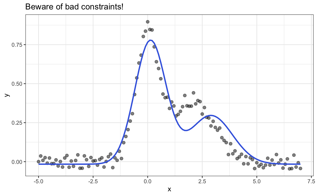
13.3.3 A more robust version of nls
Sometimes, nls() will struggle to converge towards a solution, especially if you provide initial guesses that are too far from the expected values.
fit3 <- nls(data = df,
            y ~ myfunc(x, y0, x1, x2, A1, A2, sd1, sd2),
            start = list(y0 = 0, x1 = 1, x2 = 5,
                         sd1 = .2, sd2 = .2, A1 = 10, A2 = 10)
            )
#> Error in numericDeriv(form[[3L]], names(ind), env, central = nDcentral): Missing value or an infinity produced when evaluating the modelIn that case, you may want to use a more robust nls() function such as nlsLM() from the minpack.lm package.
library(minpack.lm)
fit_nlsLM <- nlsLM(data = df,
                   y ~ myfunc(x, y0, x1, x2, A1, A2, sd1, sd2),
                   start = list(y0 = 0, x1 = 1, x2 = 5,
                                sd1 = .2, sd2 = .2, A1 = 10, A2 = 10)
                   )
summary(fit_nlsLM)
#>
#> Formula: y ~ myfunc(x, y0, x1, x2, A1, A2, sd1, sd2)
#>
#> Parameters:
#> Estimate Std. Error t value Pr(>|t|)
#> y0 0.003066 0.003702 0.828 0.409
#> x1 0.001729 0.012639 0.137 0.891
#> x2 1.959161 0.046244 42.365 <2e-16 ***
#> sd1 0.497151 0.012364 40.209 <2e-16 ***
#> sd2 1.009806 0.047403 21.303 <2e-16 ***
#> A1 0.987397 0.035369 27.917 <2e-16 ***
#> A2 1.007226 0.045414 22.179 <2e-16 ***
#> ---
#> Signif. codes: 0 '***' 0.001 '**' 0.01 '*' 0.05 '.' 0.1 ' ' 1
#>
#> Residual standard error: 0.02923 on 114 degrees of freedom
#>
#> Number of iterations to convergence: 16
#> Achieved convergence tolerance: 1.49e-08Also, nlsLM() won’t fail when the fit is exact, whereas nls() will:
testdf <- tibble(x = seq(-10,10),
                 y = dnorm(x))
nls(data = testdf,
    y ~ A*dnorm(x, sd=B, mean=x0) + y0,
    start = list(y0=0, x0=0, A=1, B=1)
    )
#> Error in nls(data = testdf, y ~ A * dnorm(x, sd = B, mean = x0) + y0, : number of iterations exceeded maximum of 50#> Nonlinear regression model
#> model: y ~ A * dnorm(x, sd = B, mean = x0) + y0
#> data: testdf
#> y0 x0 A B
#> 0 0 1 1
#> residual sum-of-squares: 0
#>
#> Number of iterations to convergence: 1
#> Achieved convergence tolerance: 1.49e-0813.4 The broom library
Thanks to the broom library, it is easy to retrieve all the fit parameters in a tibble:
#> # A tibble: 7 × 5
#>   term  estimate std.error statistic  p.value
#>   <chr>    <dbl>     <dbl>     <dbl>    <dbl>
#> 1 y0     0.00307   0.00370     0.828 4.09e- 1
#> 2 x1     0.00173   0.0126      0.137 8.91e- 1
#> 3 x2     1.96      0.0462     42.4   1.33e-71
#> 4 sd1    0.497     0.0124     40.2   3.56e-69
#> 5 sd2    1.01      0.0474     21.3   1.49e-41
#> 6 A1     0.987     0.0354     27.9   8.64e-53
#> 7 A2     1.01      0.0454     22.2   3.66e-43
# Get the fitted curve and residuals next to the original data
augment(fit_nls)#> # A tibble: 121 × 4
#> x y .fitted .resid
#> <dbl> <dbl> <dbl> <dbl>
#> 1 -5 0.0190 0.00307 0.0160
#> 2 -4.9 -0.0180 0.00307 -0.0210
#> 3 -4.8 0.0477 0.00307 0.0446
#> 4 -4.7 -0.0416 0.00307 -0.0447
#> 5 -4.6 -0.0373 0.00307 -0.0404
#> 6 -4.5 0.00699 0.00307 0.00392
#> 7 -4.4 0.0197 0.00307 0.0166
#> 8 -4.3 -0.0133 0.00307 -0.0164
#> 9 -4.2 -0.0135 0.00307 -0.0165
#> 10 -4.1 -0.0456 0.00307 -0.0487
#> # ℹ 111 more rowsIt is then easy to make a recursive fit on your data without using a for loop, like so:
library(broom)
library(tidyverse)
library(ggplot2)
theme_set(theme_bw())
# Create fake data
a <- seq(-10,10,.1)
centers <- c(-2*pi,pi,pi/6)
widths  <- runif(3, min=0.5, max=1)
amp     <- runif(3, min=2, max=10)
noise   <- .3*runif(length(a))-.15
d <- tibble(x=rep(a,3),
            y=c(amp[1]*dnorm(a,mean=centers[1],sd=widths[1])+sample(noise),
                amp[2]*dnorm(a,mean=centers[2],sd=widths[2])+sample(noise),
                amp[3]*dnorm(a,mean=centers[3],sd=widths[3])+sample(noise)),
            T=rep(1:3, each=length(a))
            )
# Plot the data
d |> ggplot(aes(x=x, y=y, color=factor(T))) +
    geom_point()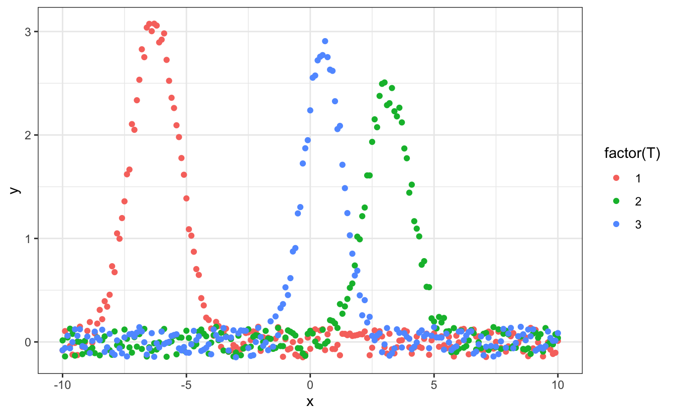
# Fit all data
d_fitted <- d |>
    nest(data = -T) |>
    mutate(fit = map(data, ~ nls(data = .,
                     y ~ y0 + A*dnorm(x, mean=x0, sd=FW),
                     start=list(A  = max(.$y),
                                y0 = .01,
                                x0 = .$x[which.max(.$y)],
                                FW = .7)
                     )),
           tidied = map(fit, tidy),
           augmented = map(fit, augment)
          )
d_fitted
#> # A tibble: 3 × 5
#> T data fit tidied augmented
#> <int> <list> <list> <list> <list>
#> 1 1 <tibble [201 × 2]> <nls> <tibble [4 × 5]> <tibble [201 × 4]>
#> 2 2 <tibble [201 × 2]> <nls> <tibble [4 × 5]> <tibble [201 × 4]>
#> 3 3 <tibble [201 × 2]> <nls> <tibble [4 × 5]> <tibble [201 × 4]>In case you want to provide fit parameters that vary depending on the group you are looking at, use the notation .$column_name, like is done here.
Then you can see the results for all your data at once:
# data and fit resulting curve
d_fitted |>
  unnest(augmented)
#> # A tibble: 603 × 8
#> T data fit tidied x y .fitted .resid
#> <int> <list> <list> <list> <dbl> <dbl> <dbl> <dbl>
#> 1 1 <tibble [201 × 2]> <nls> <tibble> -10 0.0962 -0.00445 0.101
#> 2 1 <tibble [201 × 2]> <nls> <tibble> -9.9 -0.0991 -0.00438 -0.0947
#> 3 1 <tibble [201 × 2]> <nls> <tibble> -9.8 0.136 -0.00426 0.141
#> 4 1 <tibble [201 × 2]> <nls> <tibble> -9.7 0.0940 -0.00407 0.0981
#> 5 1 <tibble [201 × 2]> <nls> <tibble> -9.6 0.0620 -0.00375 0.0658
#> 6 1 <tibble [201 × 2]> <nls> <tibble> -9.5 -0.142 -0.00324 -0.139
#> 7 1 <tibble [201 × 2]> <nls> <tibble> -9.4 0.0365 -0.00244 0.0389
#> 8 1 <tibble [201 × 2]> <nls> <tibble> -9.3 0.123 -0.00118 0.124
#> 9 1 <tibble [201 × 2]> <nls> <tibble> -9.2 -0.0240 0.000737 -0.0248
#> 10 1 <tibble [201 × 2]> <nls> <tibble> -9.1 0.00242 0.00363 -0.00121
#> # ℹ 593 more rows# fit parameters
d_fitted |>
unnest(tidied)#> # A tibble: 12 × 9
#> T data fit term estimate std.error statistic p.value augmented
#> <int> <list> <list> <chr> <dbl> <dbl> <dbl> <dbl> <list>
#> 1 1 <tibble> <nls> A 6.98 0.0614 114. 1.84e-181 <tibble>
#> 2 1 <tibble> <nls> y0 -0.00454 0.00661 -0.687 4.93e- 1 <tibble>
#> 3 1 <tibble> <nls> x0 -6.29 0.00730 -861. 0 <tibble>
#> 4 1 <tibble> <nls> FW 0.810 0.00763 106. 7.74e-176 <tibble>
#> 5 2 <tibble> <nls> A 4.36 0.0623 70.0 4.38e-141 <tibble>
#> 6 2 <tibble> <nls> y0 -0.00178 0.00660 -0.269 7.88e- 1 <tibble>
#> 7 2 <tibble> <nls> x0 3.16 0.0122 259. 1.13e-251 <tibble>
#> 8 2 <tibble> <nls> FW 0.835 0.0127 65.6 8.11e-136 <tibble>
#> 9 3 <tibble> <nls> A 4.07 0.0463 87.9 4.79e-160 <tibble>
#> 10 3 <tibble> <nls> y0 0.000980 0.00632 0.155 8.77e- 1 <tibble>
#> 11 3 <tibble> <nls> x0 0.529 0.00615 86.0 3.69e-158 <tibble>
#> 12 3 <tibble> <nls> FW 0.503 0.00630 79.8 6.12e-152 <tibble># fit parameters as a wide table
d_fitted |>
unnest(tidied) |>
select(T, term, estimate, std.error) |>
pivot_wider(names_from = term,
values_from = c(estimate,std.error))#> # A tibble: 3 × 9
#> T estimate_A estimate_y0 estimate_x0 estimate_FW std.error_A std.error_y0
#> <int> <dbl> <dbl> <dbl> <dbl> <dbl> <dbl>
#> 1 1 6.98 -0.00454 -6.29 0.810 0.0614 0.00661
#> 2 2 4.36 -0.00178 3.16 0.835 0.0623 0.00660
#> 3 3 4.07 0.000980 0.529 0.503 0.0463 0.00632
#> # ℹ 2 more variables: std.error_x0 <dbl>, std.error_FW <dbl># plot fit result
d_fitted |>
unnest(augmented) |>
ggplot(aes(x=x, color=factor(T)))+
geom_point(aes(y=y), alpha=0.5, size=3) +
geom_line(aes(y=.fitted))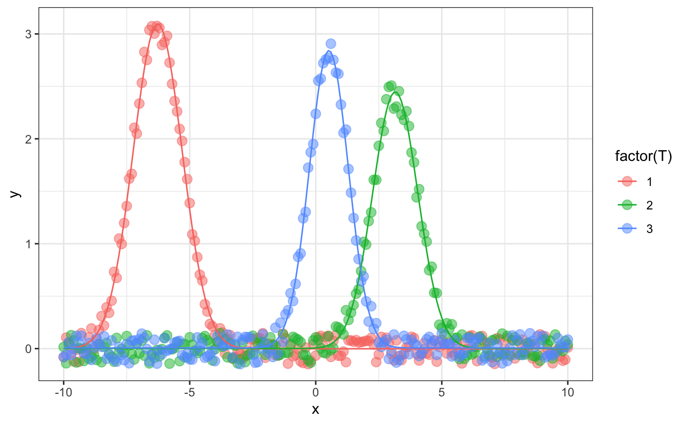
# plot fit parameters
d_fitted |>
  unnest(tidied) |>
  ggplot(aes(x=T, y=estimate, color=term))+
    geom_point()+
    geom_errorbar(aes(ymin=estimate-std.error,
                      ymax=estimate+std.error),
                  width=.1)+
    facet_wrap(~term, scales="free_y")+
    theme(legend.position = "none")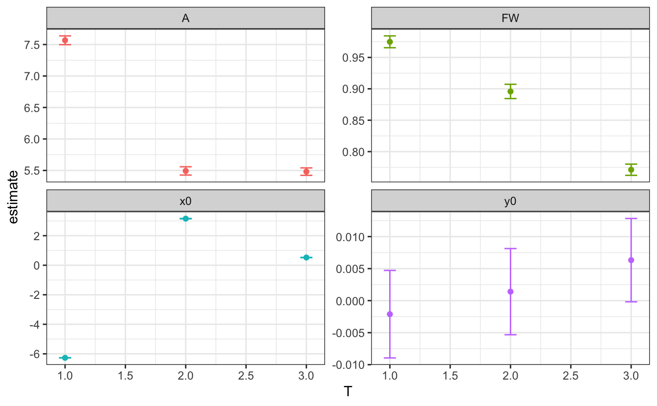
13.5 Exercises
Download the exercises and solutions from the following repositories, then create a Rstudio project from the unzipped folder:
Exercise 1
- Load exo_fit.txt in a
tibble. - Using
lm()ornls()fit each column as a function ofxand display the “experimental” data and the fit on the same graph.- Tip: Take a look at the function
dnorm()to define a Gaussian
- Tip: Take a look at the function
Exercise 2
- Load the
tidyverselibrary. - Define a function
norm01(x), that, given a vectorx, returns this vector normalized to [0,1]. - Load the Raman spectrum rubis_01.txt, normalize it to [0,1] and plot it
- Define the normalized Lorentzian function
Lorentzian(x, x0, FWHM), defined by \(L(x, x_0, FWHM)=\frac{FWHM}{2\pi}\frac{1}{(FWHM/2)^2 + (x-x_0)^2}\) - Guess grossly the initial parameters and plot the resulting curve as a blue dashed line
- Fit the data by a sum of 2 Lorentzians using
nls() - Add the result on the plot as a red line
- Add the 2 Lorentzian components as area-filled curves with
alpha=0.2and two different colors
Solution
# Load the `tidyverse` library.
library(tidyverse)
# Define a function `norm01(x)`, that, given a vector `x`, returns this vector normalized to [0,1].
norm01 <- function(x) {(x-min(x))/(max(x)-min(x))}
# Load rubis_1.txt, normalize it to [0,1] and plot it
d <- read_table("Data/rubis_01.txt", col_names=c("w", "Int")) |>
    mutate(Int_n = norm01(Int))
P <- d |>
    ggplot(aes(x=w, y=Int_n))+
        geom_point(alpha=0.5)
P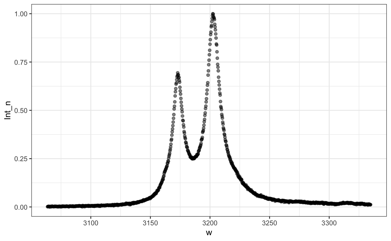
# Define the Lorentzian function
Lorentzian <- function(x, x0=0, FWHM=1){
    FWHM / (2*pi) / ((FWHM/2)^2 + (x - x0)^2)
}
# Guess grossly the initial parameters and plot the resulting curve as a blue dashed line
P+geom_line(aes(y = 0.03 +
                    3*Lorentzian(w, x0=3160, FWHM=10) +
                    7*Lorentzian(w, x0=3210, FWHM=10)),
            col="blue", lty=2)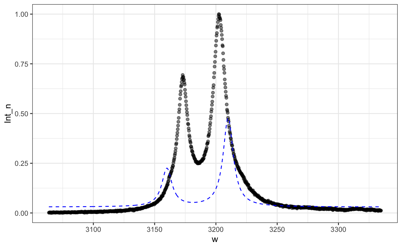
# Fit the data by a sum of 2 Lorentzians using `nls`
fit <- nls(data=d,
           Int_n ~ y0 + A1*Lorentzian(w,x1,FWHM1) + A2*Lorentzian(w,x2,FWHM2),
           start=list(y0=0.03,
                      x1=3160, FWHM1=10, A1=3,
                      x2=3200, FWHM2=10, A2=7))
summary(fit)
#>
#> Formula: Int_n ~ y0 + A1 * Lorentzian(w, x1, FWHM1) + A2 * Lorentzian(w,
#> x2, FWHM2)
#>
#> Parameters:
#> Estimate Std. Error t value Pr(>|t|)
#> y0 9.825e-03 6.165e-04 15.94 <2e-16 ***
#> x1 3.173e+03 3.503e-02 90576.82 <2e-16 ***
#> FWHM1 1.076e+01 1.087e-01 98.96 <2e-16 ***
#> A1 1.039e+01 8.028e-02 129.38 <2e-16 ***
#> x2 3.203e+03 2.709e-02 118214.68 <2e-16 ***
#> FWHM2 1.453e+01 8.600e-02 169.00 <2e-16 ***
#> A2 2.112e+01 9.680e-02 218.19 <2e-16 ***
#> ---
#> Signif. codes: 0 '***' 0.001 '**' 0.01 '*' 0.05 '.' 0.1 ' ' 1
#>
#> Residual standard error: 0.01568 on 1008 degrees of freedom
#>
#> Number of iterations to convergence: 10
#> Achieved convergence tolerance: 7.652e-06# Add the result on the plot as a red line
P + geom_line(aes(y=.03 +
3*Lorentzian(w, x0=3160, FWHM=10) +
7*Lorentzian(w, x0=3210, FWHM=10)),
col="blue", lty=2)+
geom_line(aes(y=predict(fit)), col="red")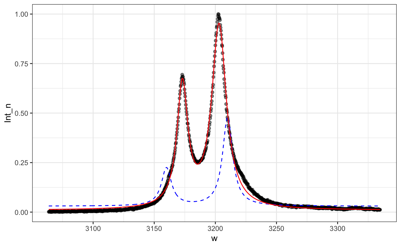
# Add the 2 Lorentzian components as area-filled curves with `alpha=0.2` and two different colors
y0  <- coef(fit)['y0']
A1  <- coef(fit)['A1'];   A2   <- coef(fit)['A2']
x1  <- coef(fit)['x1'];   x2   <- coef(fit)['x2']
FW1 <- coef(fit)['FWHM1']; FW2 <- coef(fit)['FWHM2']
P + geom_line(aes(y=.03 +
                    3*Lorentzian(w, x0=3160, FWHM=10) +
                    7*Lorentzian(w, x0=3210, FWHM=10)),
            col="blue", lty=2)+
    geom_line(aes(y = predict(fit)), col="red")+
    geom_area(aes(y = A1*Lorentzian(w, x0=x1, FWHM=FW1)),
                fill="royalblue", alpha=.2)+
    geom_area(aes(y = A2*Lorentzian(w, x0=x2, FWHM=FW2)),
                fill="orange", alpha=.2)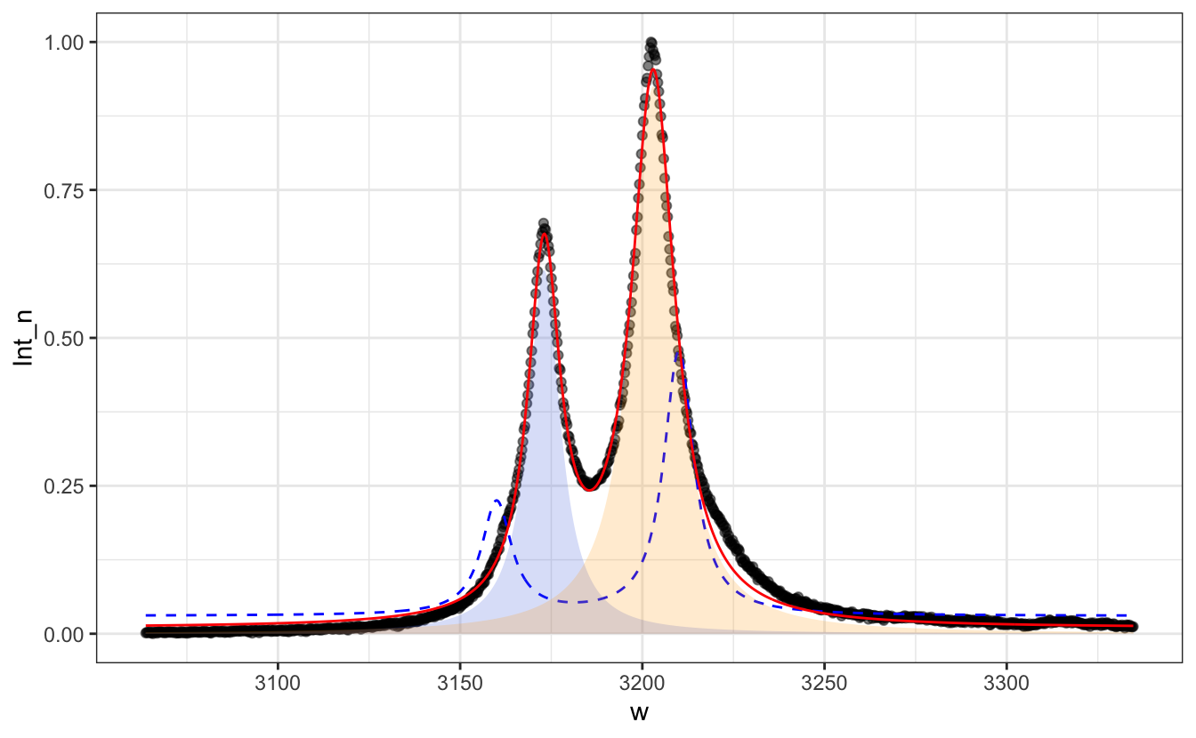
Exercise 3
- Create an
Exercise_fitfolder, and create an Rstudio project linked to this folder -
Download the corresponding data files and unzip them in a folder called
Data. - Create a new .R file in which you will write your code and save it.
- Like in the previous exercise, we will fit ruby Raman spectra, but we will do it on many files at once. First, using
list.files(), save inflistthe list of ruby files in theDatafolder. - Define the
Lorentzian(x, x0, FWHM)function - Define the
norm01(x)function returning the vector x normalized to [0,1] - Create a
read_ruby(filename)function that, given a file namefilename, reads the file into a tibble, gives the proper column names, normalizes the intensity to [0,1], and returns the tibble. - Create a
fitfunc(tib)function that, given a tibbletib, fits this tibble’s y values as a function of the x values using the sum of two Lorentzians, and returns thenls()fit result. Make sure to provide “clever” starting parameters, especially for the positions of the two peaks. For example, one peak is where the spectrum maximum is, and the other one is always at an energy roughly 30 cm-1 lower. - Using pipe operations and
map(), recursively:- Create a tibble with only one column called
file, which contains the list of file namesflist. - Create a column
datacontaining a list of all read files, obtained by mappingread_ruby()ontoflist. - Create a column
fitcontaining a list ofnls()objects, obtained by mappingfitfunc()onto the list (column)data - Create a column
tidiedcontaining a list of tidiednls()tibbles, obtained by mappingbbroom::tidy()onto the list (column)fit - Create a column
augmentedcontaining a list of augmentednls()tibbles, obtained by mappingbbroom::augment()onto the list (column)fit - Turn the
filecolumn intorunthat will contain the run number (i.e. the number in the file name) as a numeric value. Use the functionseparate()to do so.
- Create a tibble with only one column called
- Plot all the experimental data and the fit with black points and red lines into a faceted plot. Play with various ways of plotting this, like a ridge or slider plot.
- Plot the evolution of all fitting parameters as a function of the run number.
- Plot the evolution of the position of the higher energy peak as a function of the file name.
- Fit linearly the evolution of the higher intensity peaks with respect to the run number. Display the fitted parameters and R2. Plot the fit as a red line. Make sure to use proper weighing for the fit.
Solution
# - Using `list.files()`, save in `flist` the list of ruby files in the `Data` folder.
flist <- list.files(path = "Data", pattern = "rubis", full.names = TRUE)
# - Define the `Lorentzian(x, x0, FWHM)` function
Lorentzian <- function(x, x0 = 0, FWHM = 1) {
    2 / (pi * FWHM) / (1 + ((x - x0) / (FWHM / 2))^2)
}
# - Define the `norm01(x)` function returning the vector x normalized to [0,1]
norm01 <- function(x) {
    (x - min(x)) / (max(x) - min(x))
}
# - Create a `read_ruby(filename)` function that, given a file name `filename`,
# reads the file into a tibble, gives the proper column names, normalizes the
# intensity to [0,1], and returns the tibble.
read_ruby <- function(filename){
    read_table(filename, col_names = c("w", "Int")) |>
        mutate(Int = norm01(Int))
}
# - Create a `fitfunc(tib)` function that, given a tibble `tib`, fits this
# tibble's *y* values as a function of the *x* values using the sum of two Lorentzians,
# and returns the `nls()` fit result. Make sure to provide "clever" starting parameters,
# especially for the positions of the two peaks. For example, one peak is where
# the spectrum maximum is, and the other one is always at an energy roughly 30 cm^-1^ lower.
fitfunc <- function(tib){
    nls(data=tib,
        Int ~ y0 + A1*Lorentzian(w,x1,FWHM1)+
                   A2*Lorentzian(w,x2,FWHM2),
           start=list(y0=0.03,
                      x1=tib$w[which.max(tib$Int)] - 30,
                      FWHM1=10,
                      A1=max(tib$Int)*10,
                      x2=tib$w[which.max(tib$Int)],
                      FWHM2=10,
                      A2=max(tib$Int)*10)
        )
}
# Test it:
# df <- read_ruby(flist[1])
# fitfunc(df)
#
# - Using pipe operations and `map()`, recursively:
#     - Create a tibble with only one column called `file`, which contains the
#       list of file names `flist`.
#     - Create a column `data` containing a list of all read files,
#       obtained by mapping `read_ruby()` onto `flist`.
#     - Create a column `fit` containing a list of `nls()` objects,
#       obtained by mapping `fitfunc()` onto the list (column) `data`
#     - Create a column `tidied` containing a list of tidied `nls()` tibbles,
#       obtained by mapping `bbroom::tidy()` onto the list (column) `fit`
#     - Create a column `augmented` containing a list of augmented `nls()` tibbles,
#       obtained by mapping `bbroom::augment()` onto the list (column) `fit`
#     - Turn the `file` column into `run` that will contain the run number
#       (*i.e.* the number in the file name) as a numeric value.
#       Use the function `separate()`{.R} to do so.
data <- tibble(file=flist) |>
    mutate(data = map(file, read_ruby),
           fit = map(data, fitfunc),
           tidied = map(fit, tidy),
           augmented = map(fit, augment)
           ) |>
    separate(file, c(NA, NA, "run", NA), convert = TRUE)
# - Plot all the experimental data and the fit with black points and red lines
# into a faceted plot. Play with various ways of plotting this,
# like a ridge or slider plot.
data |>
    unnest(augmented) |>
    ggplot(aes(x = w, y = Int)) +
       geom_point(alpha=0.5)+
       geom_line(aes(y=.fitted), col="red")+
       facet_wrap(~run)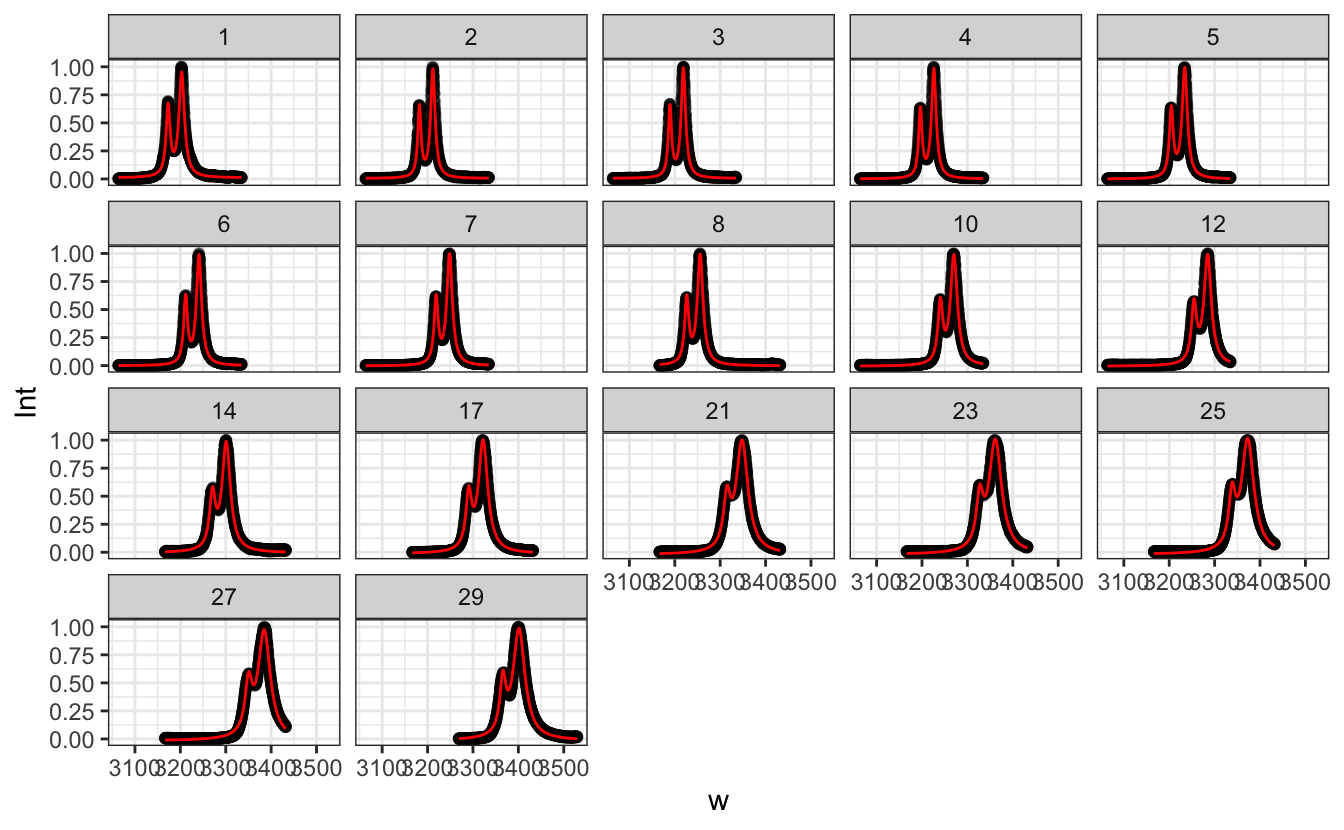
data |>
    unnest(augmented) |>
    ggplot(aes(x = w, y = Int + as.numeric(factor(run)), group=run)) +
       geom_point(alpha=0.5)+
       geom_line(aes(y = .fitted + as.numeric(factor(run))), col = "red")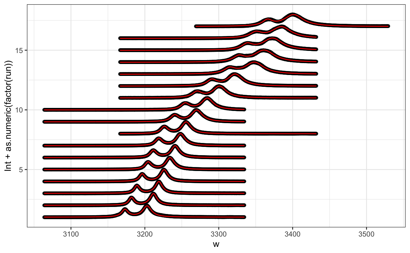
P <- data |>
    unnest(augmented) |>
    ggplot(aes(x = w, y = Int, frame=run)) +
        geom_point(alpha = 0.5) +
        geom_line(aes(y = .fitted), col = "red")
library(plotly)
ggplotly(P, dynamicTicks = TRUE) |>
    animation_opts(5)|>
    layout(xaxis = list(autorange=FALSE, range = c(3050, 3550)))
# - Plot the evolution of all fitting parameters as a function of the run number.
data |>
unnest(tidied) |>
ggplot(aes(x = run, y = estimate)) +
geom_point()+
facet_wrap(~term, scales = "free")+
geom_errorbar(aes(ymin = estimate - std.error,
ymax = estimate + std.error),
width=0.5)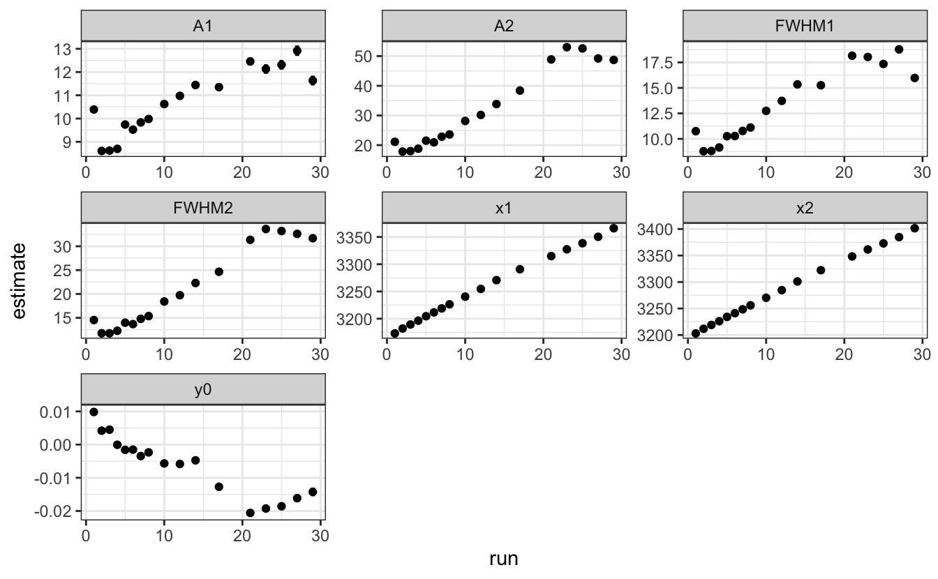
# - Plot the evolution of the position of the higher intensity peaks.
data |>
    unnest(tidied) |>
    filter(term == "x1") |>
    ggplot(aes(x = run, y = estimate)) +
        geom_point()+
        geom_errorbar(aes(ymin = estimate - std.error,
                          ymax = estimate + std.error),
                      width=0.5)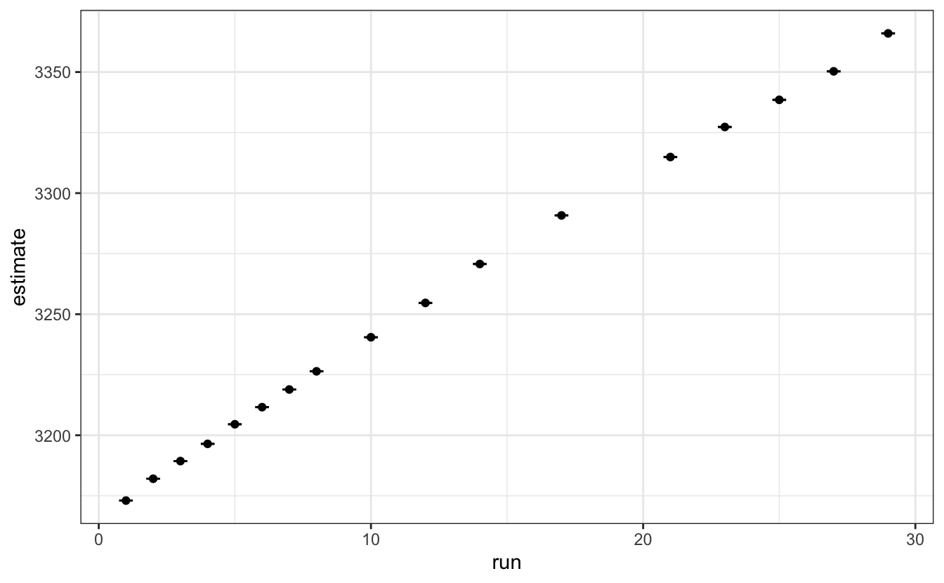
# - Fit linearly the evolution of the higher intensity peaks with respect to the
#   run number. Display the fitted parameters and R^2^.Plot the fit as a red line.
#   Make sure to use proper weighing for the fit.
lmfit <- data |>
    unnest(tidied) |>
    filter(term == "x1") |>
    lm(data=_,
       estimate ~ run,
       weights = 1/std.error^2)
tidy(lmfit)
#> # A tibble: 2 × 5
#> term estimate std.error statistic p.value
#> <chr> <dbl> <dbl> <dbl> <dbl>
#> 1 (Intercept) 3169. 0.557 5686. 6.39e-49
#> 2 run 6.99 0.0756 92.6 4.23e-22glance(lmfit)#> # A tibble: 1 × 12
#> r.squared adj.r.squared sigma statistic p.value df logLik AIC BIC
#> <dbl> <dbl> <dbl> <dbl> <dbl> <dbl> <dbl> <dbl> <dbl>
#> 1 0.998 0.998 57.6 8566. 4.23e-22 1 -36.0 78.1 80.6
#> # ℹ 3 more variables: deviance <dbl>, df.residual <int>, nobs <int>data |>
unnest(tidied) |>
filter(term == "x1") |>
ggplot(aes(x = run, y = estimate)) +
geom_point()+
geom_errorbar(aes(ymin = estimate - std.error,
ymax = estimate + std.error),
width=0.5)+
geom_line(aes(y = predict(lmfit)), col="red")