You may want to plot your data as a color map, like the evolution of a Raman spectrum as a function of temperature, pressure or position. In some cases you’ll have a 3-columns data.frame with x, y, and z values (e.g. intensity of a peak as a function of the position on the sample), in some cases you can have a list of spectra evolving with a given parameter.
12.1 The ggplot2 solution
Let’s create a dummy set of spectra that we will gather in a tidy tibble.
library(tidyverse)Nspec<-40# Amount of spectraN<-500# Size of the x vector# Create a fake data tibblefake_data<-tibble(T =round(seq(273, 500, length=Nspec), 1))|>mutate(spec =map(T, ~tibble(w =seq(0, 100, length =N), Intensity =50*dnorm(w, mean =(./T[1])*20+25, sd =10+runif(1,max=5)))))fake_data
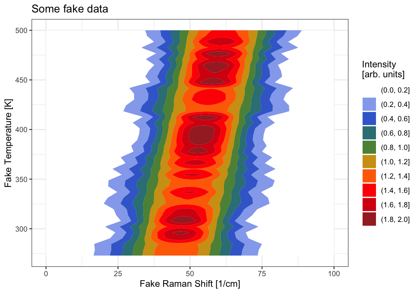
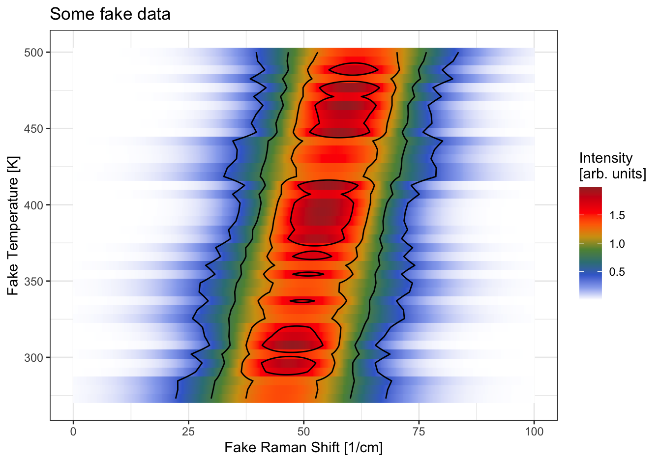
OK, so now we have some fake experimental data stored in a tidy tibble called fake_data. We want to plot it as a color map in order to grasp the evolution of the spectra. This can be done through the use of geom_contour() and geom_contour_filled() functions and by providing the z aesthetics, or by using the geom_raster() or geom_tile() functions with a fill aesthetics. Both methods can be combined, as shown below:
# Plottingcolors<-colorRampPalette(c("white","royalblue","seagreen","orange","red","brown"))Nbins<-10ggplot(data=fake_data, aes(x=w, y=T, z=Intensity))+geom_contour_filled(bins =Nbins)+ggtitle("Some fake data")+scale_fill_manual(values =colors(Nbins), name ="Intensity\n[arb. units]")+labs(x ="Fake Raman Shift [1/cm]", y ="Fake Temperature [K]")+theme_bw()
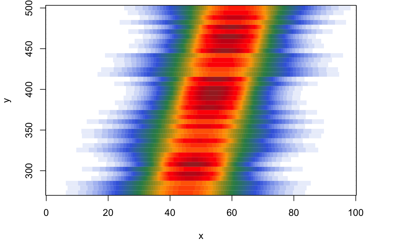
In some cases you end up with a matrix z, and two vectors x and y. This is easy to plot using the base image() function. For the sake of example, let’s just pivot our 3-columns data.frame to such a matrix using pivot_wider():
x<-sort(unique(fake_data$w))y<-sort(unique(fake_data$T))z<-as.matrix(fake_data|>pivot_wider(values_from =Intensity, names_from =T)|>select(-w))colors<-colorRampPalette(c("white","royalblue","seagreen","orange","red","brown"))(50)par(mar =c(4, 4, .5, 4), lwd =2)image(x, y, z, col =colors)
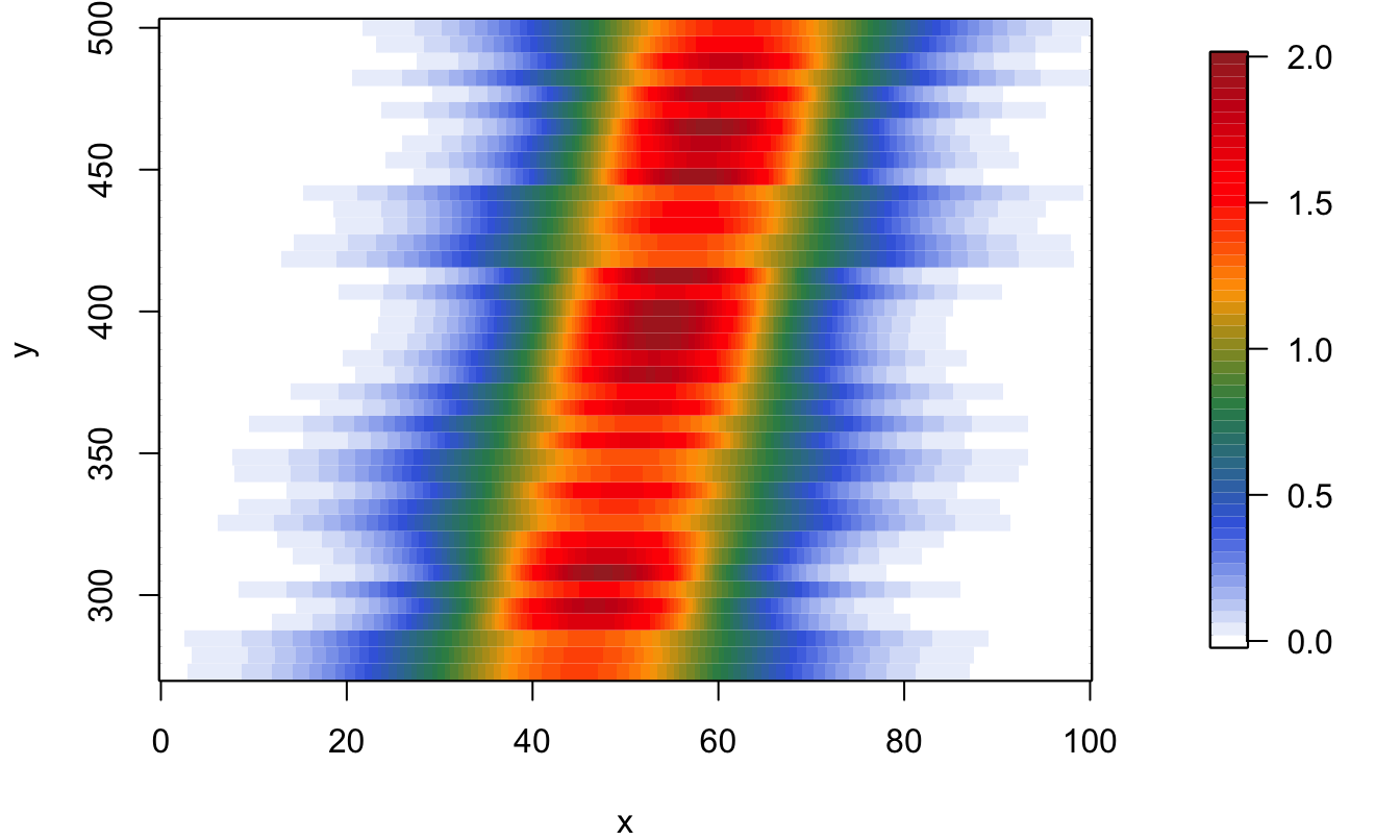
You can add a legend by using the image.plot function:
And finally, if you want to make this an interactive plot, you can use plot_ly():
library(plotly)aX<-list(title ="Raman Shift [1/cm]")aY<-list(title ="Temperature [K]")# Weird but you need to use t(z) here:z<-t(z)# Color plotplot_ly(x =x, y =y, z =z, type ="heatmap", colors =colors)|>layout(xaxis =aX, yaxis =aY)
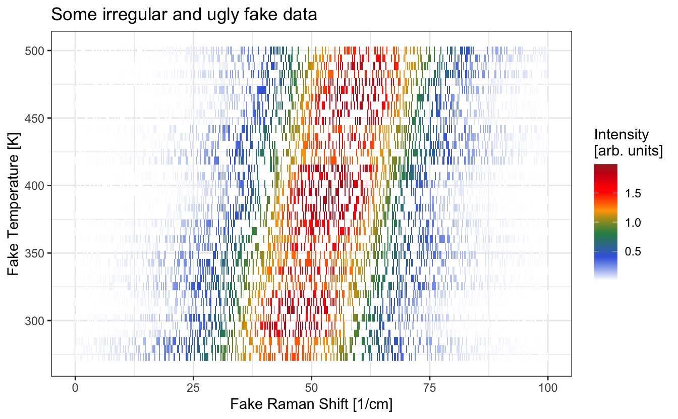
In case you have a set of non-regular data, plotting it as a color map can get tricky: how do we tell the plotting device what color should be in a place where there is no data point?
The solution is to use a spline (or linear, but spline looks usually nicer) interpolation of your 2D data. For this, we can use the akima package and its interp() function, like so:
# let's make our data irregular and see the plot is now not working:irreg.df<-fake_data[sample(nrow(fake_data), nrow(fake_data)/3),]# let's plot these irregular datacolors<-colorRampPalette(c("white","royalblue","seagreen","orange","red","brown"))(500)ggplot(data=irreg.df, aes(x=w, y=T, fill=Intensity))+geom_raster()+#geom_tile would workggtitle("Some irregular and ugly fake data")+scale_fill_gradientn(colors=colors,name="Intensity\n[arb. units]")+labs(x ="Fake Raman Shift [1/cm]", y ="Fake Temperature [K]")+theme_bw()
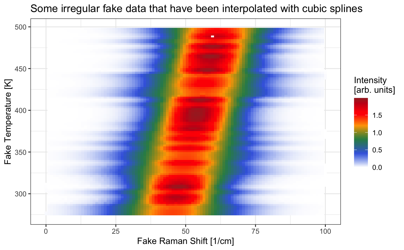
# now let's interpolate the data on a 100x100 regular grid# linear = FALSE -> cubic interpolationlibrary(akima)irreg.df.interp<-with(irreg.df, interp(x=w, y=T, z=Intensity, nx =100, ny =100, duplicate ="median", extrap =FALSE, linear =FALSE))# irreg.df.interp is a list of 2 vectors and a matrixstr(irreg.df.interp)
#> List of 3
#>  $ x: num [1:100] 0 1.01 2.02 3.03 4.04 ...
#>  $ y: num [1:100] 273 275 278 280 282 ...
#>  $ z: num [1:100, 1:100] NaN NaN NaN NaN NaN NaN NaN NaN NaN NaN ...
# Regrouping this list to a 3-columns data.frameirreg.df.smooth<-expand.grid(w =irreg.df.interp$x, T =irreg.df.interp$y)|>tibble()|>mutate(Intensity =as.vector(irreg.df.interp$z))|>na.omit()# Plottingirreg.df.smooth|>ggplot(aes(x=w, y=T, fill=Intensity))+geom_raster()+ggtitle("Some irregular fake data that have been interpolated with cubic splines")+scale_fill_gradientn(colors=colors, name="Intensity\n[arb. units]")+labs(x ="Fake Raman Shift [1/cm]", y ="Fake Temperature [K]")+theme_bw()
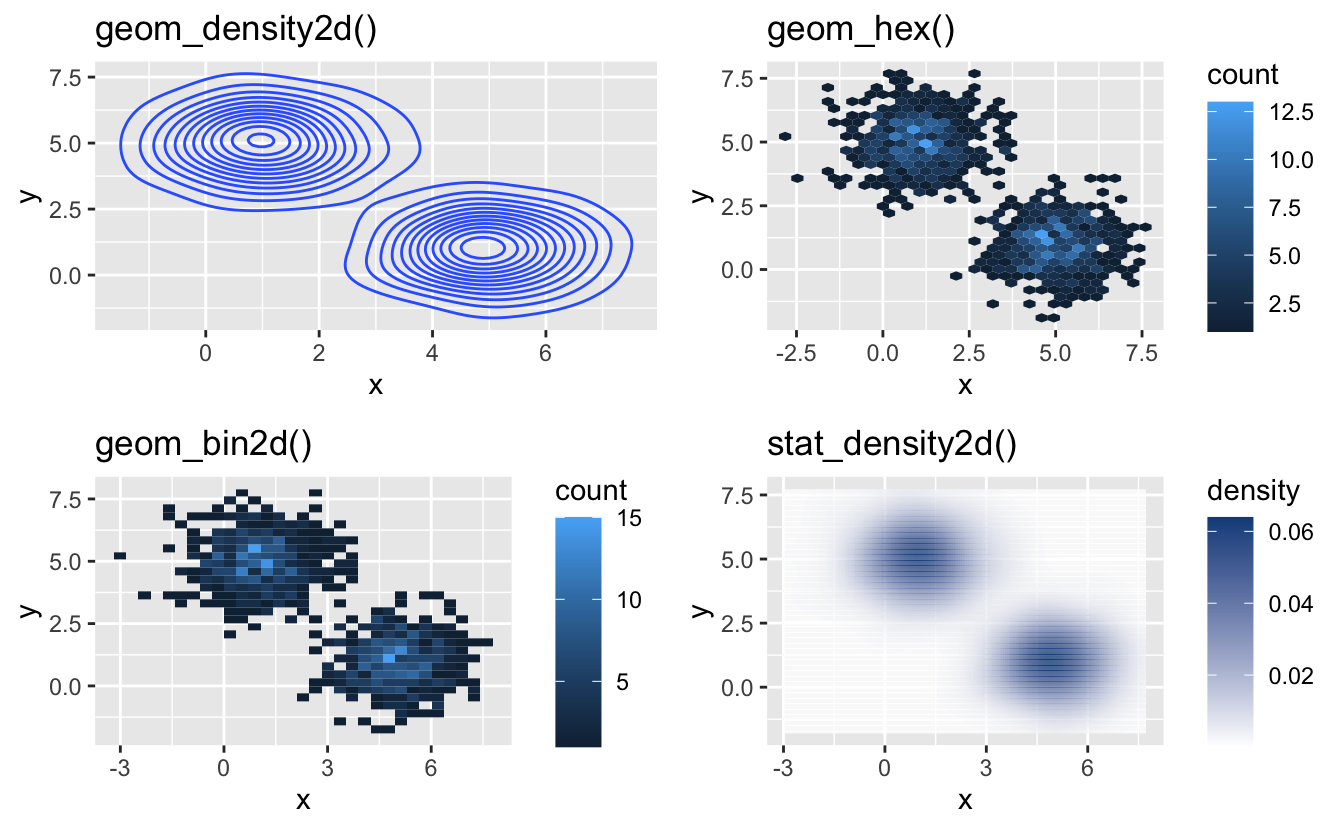
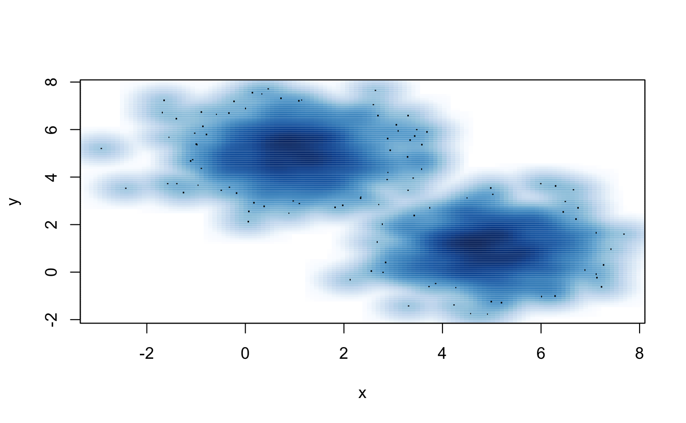
12.5 2D density of points
In case you want to plot a density of points, you have a variety of solutions:
# 3D color plots {#colorplots}```{r include=FALSE, warning=FALSE, message=FALSE}detachAllPackages <- function() { basic.packages <- c("package:stats","package:graphics","package:grDevices","package:utils","package:datasets","package:methods","package:base") package.list <- search()[ifelse(unlist(gregexpr("package:",search()))==1,TRUE,FALSE)] package.list <- setdiff(package.list,basic.packages) if (length(package.list)>0) for (package in package.list) detach(package, character.only=TRUE)}detachAllPackages()rm(list = ls(all = TRUE))library(knitr)```You may want to plot your data as a color map, like the evolution of a Raman spectrum as a function of temperature, pressure or position. In some cases you'll have a 3-columns `data.frame`{.R} with x, y, and z values (_e.g._ intensity of a peak as a function of the position on the sample), in some cases you can have a list of spectra evolving with a given parameter. ## The ggplot2 solutionLet's create a dummy set of spectra that we will gather in a tidy `tibble`{.R}.```{r, message=FALSE}library(tidyverse)Nspec <- 40 # Amount of spectraN <- 500 # Size of the x vector# Create a fake data tibblefake_data <- tibble(T = round(seq(273, 500, length=Nspec), 1)) |> mutate(spec = map(T, ~tibble(w = seq(0, 100, length = N), Intensity = 50*dnorm(w, mean = (./T[1])*20 + 25, sd = 10+runif(1,max=5)))))fake_datafake_data <- fake_data |> unnest(spec)fake_data```OK, so now we have some fake experimental data stored in a tidy `tibble`{.R} called `fake_data`. We want to plot it as a color map in order to grasp the evolution of the spectra. This can be done through the use of `geom_contour()`{.R} and `geom_contour_filled()`{.R} functions and by providing the `z` aesthetics, or by using the `geom_raster()`{.R} or `geom_tile()`{.R} functions with a `fill` aesthetics. Both methods can be combined, as shown below:```{r, out.width='100%', warning=FALSE, message = FALSE, fig.asp=.7,cache=FALSE}# Plottingcolors <- colorRampPalette(c("white","royalblue","seagreen", "orange","red","brown"))Nbins <- 10ggplot(data=fake_data, aes(x=w, y=T, z=Intensity)) + geom_contour_filled(bins = Nbins) + ggtitle("Some fake data") + scale_fill_manual(values = colors(Nbins), name = "Intensity\n[arb. units]") + labs(x = "Fake Raman Shift [1/cm]", y = "Fake Temperature [K]") + theme_bw()ggplot(data=fake_data, aes(x = w, y = T)) + geom_raster(aes(fill = Intensity)) + #geom_tile would work geom_contour(aes(z = Intensity), color = "black", bins = 5)+ ggtitle("Some fake data") + scale_fill_gradientn(colors = colors(10), name = "Intensity\n[arb. units]") + labs(x = "Fake Raman Shift [1/cm]", y = "Fake Temperature [K]") + theme_bw()```Another option is to make a "ridge plot", or a stacking of plots:```{r, out.width='100%', message = FALSE, fig.asp=.7,cache=FALSE}colors <- colorRampPalette(c("royalblue","seagreen","orange", "red","brown"))(length(unique(fake_data$T)))ggplot(data = fake_data, aes(x = w, y = Intensity + as.numeric(factor(T))-1, color = factor(T)) ) + geom_line() + labs(x = "Fake Raman Shift [1/cm]", y = "Fake Intensity [arb. units]") + coord_cartesian(xlim = c(25,75)) + scale_color_manual(values=colors,name="Fake\nTemperature [K]") + theme_bw()ggplot(data=fake_data, aes(x = w, y = Intensity + as.numeric(factor(T))-1, color = T, group = T) )+ geom_line() + labs(x="Fake Raman Shift [1/cm]", y="Fake Intensity [arb. units]") + scale_color_gradientn(colors=colors,name="Fake\nTemperature [K]") + coord_cartesian(xlim = c(25,75)) + theme_bw()```## The base graphics solutionIn some cases you end up with a matrix _z_, and two vectors _x_ and _y_. This is easy to plot using the base `image()`{.R} function. For the sake of example, let's just pivot our 3-columns data.frame to such a matrix using `pivot_wider()`{.R}:```{r, out.width='100%', message = FALSE, warning = FALSE, fig.asp=.6,cache=FALSE}x <- sort(unique(fake_data$w))y <- sort(unique(fake_data$T))z <- as.matrix(fake_data |> pivot_wider(values_from = Intensity, names_from = T) |> select(-w) )colors <- colorRampPalette(c("white","royalblue","seagreen","orange","red","brown"))(50)par(mar = c(4, 4, .5, 4), lwd = 2)image(x, y, z, col = colors)```You can add a legend by using the `image.plot` function:```{r, out.width='100%', message = FALSE, warning = FALSE, fig.asp=.6,cache=FALSE}library(fields)par(mar=c(4, 4, .5, 4), lwd=2)image.plot(x,y,z, col = colors)```## The plotly solutionAnd finally, if you want to make this an interactive plot, you can use `plot_ly()`{.R}:```{r, out.width='100%', message = FALSE, warning = FALSE, fig.asp=.6,cache=FALSE}library(plotly)aX <- list(title = "Raman Shift [1/cm]")aY <- list(title = "Temperature [K]")# Weird but you need to use t(z) here:z <- t(z)# Color plotplot_ly(x = x, y = y, z = z, type = "heatmap", colors = colors) |> layout(xaxis = aX, yaxis = aY)```Or, very cool, an interactive surface plot:```{r, out.width='100%', message = FALSE, warning = FALSE, fig.asp=.9,cache=FALSE}plot_ly(x=x, y=y, z=z, type = "surface", colors=colors) |> layout(scene = list(xaxis = aX, yaxis = aY, dragmode="turntable"))```## The case of non-regular dataIn case you have a set of non-regular data, plotting it as a color map can get tricky: how do we tell the plotting device what color should be in a place where there is no data point?The solution is to use a spline (or linear, but spline looks usually nicer) interpolation of your 2D data. For this, we can use the `akima` package and its `interp()`{.R} function, like so:```{r include=TRUE, warning = FALSE, message=FALSE, cache=FALSE}# let's make our data irregular and see the plot is now not working:irreg.df <- fake_data[sample(nrow(fake_data), nrow(fake_data)/3),]# let's plot these irregular datacolors <- colorRampPalette(c("white","royalblue","seagreen", "orange","red","brown"))(500)ggplot(data=irreg.df, aes(x=w, y=T, fill=Intensity)) + geom_raster() + #geom_tile would work ggtitle("Some irregular and ugly fake data") + scale_fill_gradientn(colors=colors,name="Intensity\n[arb. units]") + labs(x = "Fake Raman Shift [1/cm]", y = "Fake Temperature [K]") + theme_bw()# now let's interpolate the data on a 100x100 regular grid# linear = FALSE -> cubic interpolationlibrary(akima)irreg.df.interp <- with(irreg.df, interp(x=w, y=T, z=Intensity, nx = 100, ny = 100, duplicate = "median", extrap = FALSE, linear = FALSE) )# irreg.df.interp is a list of 2 vectors and a matrixstr(irreg.df.interp)# Regrouping this list to a 3-columns data.frameirreg.df.smooth <- expand.grid(w = irreg.df.interp$x, T = irreg.df.interp$y) |> tibble() |> mutate(Intensity = as.vector(irreg.df.interp$z)) |> na.omit()# Plottingirreg.df.smooth |> ggplot(aes(x=w, y=T, fill=Intensity)) + geom_raster() + ggtitle("Some irregular fake data that have been interpolated with cubic splines") + scale_fill_gradientn(colors=colors, name="Intensity\n[arb. units]") + labs(x = "Fake Raman Shift [1/cm]", y = "Fake Temperature [K]") + theme_bw()```## 2D density of pointsIn case you want to plot a density of points, you have a variety of solutions:```{r}df <-tibble(x=rnorm(1e3, mean=c(1,5)),y=rnorm(1e3, mean=c(5,1)))p1 <-ggplot(data=df, aes(x=x,y=y))+geom_density2d() +ggtitle('geom_density2d()')p2 <-ggplot(data=df, aes(x=x,y=y))+geom_hex() +ggtitle('geom_hex()')p3 <-ggplot(data=df, aes(x=x,y=y))+geom_bin2d() +ggtitle('geom_bin2d()')p4 <-ggplot(data=df, aes(x=x,y=y))+ggtitle('stat_density2d()') +stat_density2d(aes(fill = ..density..), geom ="tile", contour =FALSE, n =200) +scale_fill_continuous(low ="white", high ="dodgerblue4")library(cowplot)plot_grid(p1,p2,p3,p4)```Or the base `smoothScatter()`{.R} function could do the trick:```{r}smoothScatter(df)```